Curo Calculator is your ultimate tool for calculating loan, lease, and hire purchase repayments and interest rates, ideal for both borrowers and finance professionals.
Our aim is to enhance your understanding of the calculator’s many useful features and perhaps shed light on financial concepts you might not have explored before.
While Curo Calculator is equipped for advanced calculations, there are specific scenarios it does not support directly:
Multiple Interest Rate Calculations:
Current Limitation: Curo Calculator does not handle scenarios where interest rates change over time, like fixed-to-variable rate mortgages, in a single step.
Solution: You can perform these calculations by breaking them down into several steps. We’ve detailed how to do this in our guide to Multiple Interest Rate Calculations. Using this method, you can calculate different segments of the loan with different rates separately and then determine the overall implicit rates (NAR and APR) with a single calculation using the advanced features of the calculator.
Early Settlement Calculations:
Current Limitation: The calculator does not support direct calculation for early settlements.
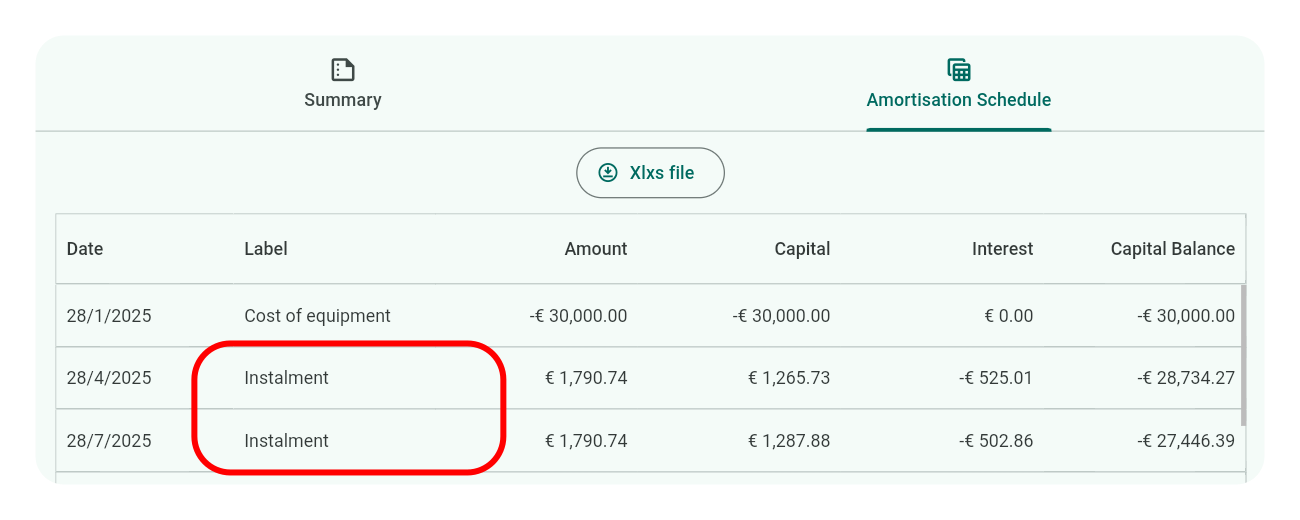
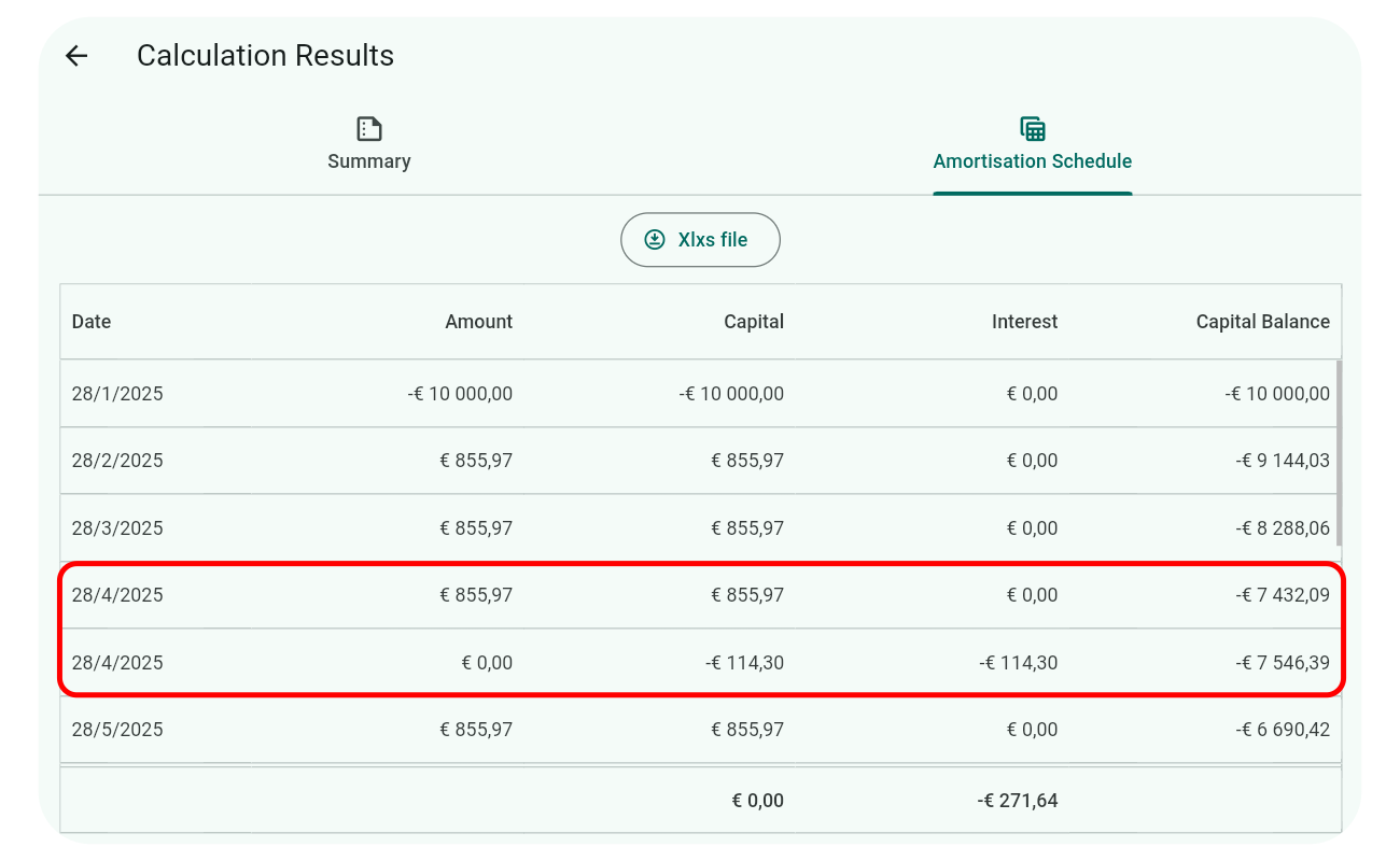
Solution: For fully amortised loans, you can still use Curo Calculator effectively by:
entering the payments made up to the current date.
adding a final payment to represent the settlement amount to calculate.
Important: Ensure that the Date Input display option setting is enabled for precise calculations.
Additionally, please note:
Taxes: The calculator does not account for taxes. Exclude VAT from your inputs where applicable, but include Sales Tax in the financing amount if relevant.
With these points clarified, why not:
Take a Quick Tour to familiarise yourself with app navigation and calculation tips.
Explore Templates to streamline your calculations.
Review our comprehensive Examples for practical applications.
Subsections of Homepage
Quick Tour
Navigation
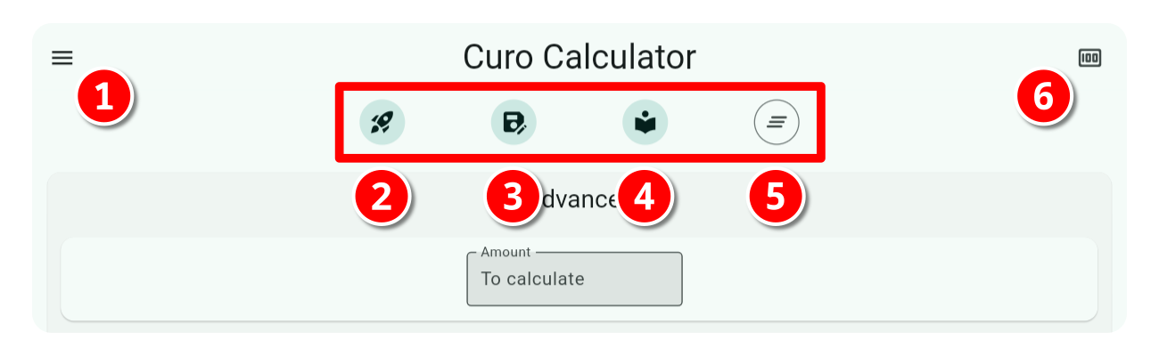
The minimalistic design of the calculator provides access to key features using one-tap selection of icons, located discreetly at the top of the input screen. These are identified 1 to 6 in the image and are described below:
App Menu Icon: Provides access to the calculator side-panel menu (covered below)
Rocket Icon: Launches a pop-up selection panel containing a list of your saved templates. Use the search feature if required, and tap on the required template to load it.
Save Icon: Launches a pop-up to capture details of the calculator input you want to save as a template. See My Templates > Creating a Template for more.
Library Icon: Launches a pop-up selection panel containing a list of built-in calculation Examples. Use the search feature if required, and tap on the required example to load it.
Clear Icon: Clears all calculation input and resets the calculator using your default settings.
Currency Icon: Launches a pop-up currency selector using the currencies defined in Settings > Currencies. Use it to switch currency input and display formats.
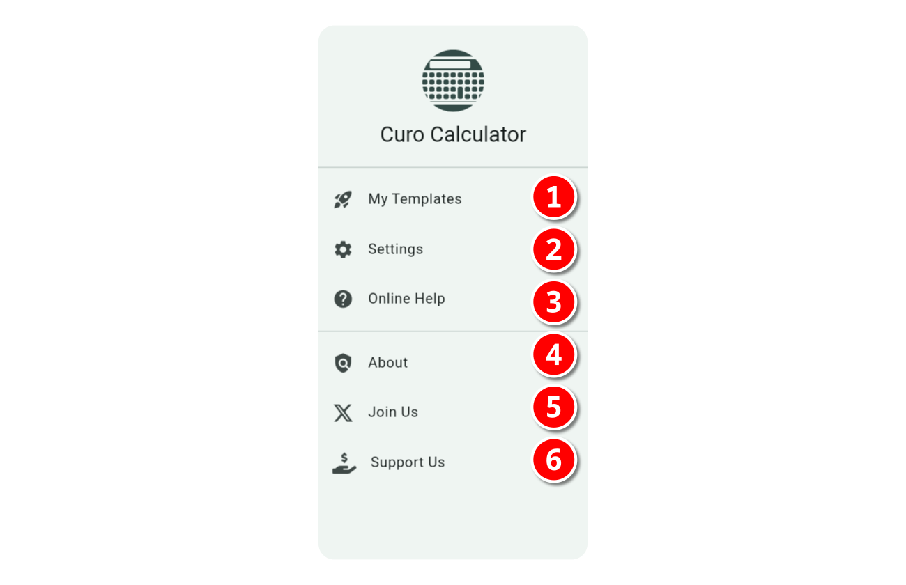
The calculator side-panel menu shown below contains menu items labelled 1 to 4 and are described below:
Settings: This is where you tailor the calculator’s layout to suit your needs, whether for straightforward daily calculations or advanced financial scenarios. See Settings for more.
Online Help: No more to add…you’re here!
About: Provides basic information about the app, including version number which is important if you are reporting a problem, and also a disclaimer which we remind you is “The application is provided as is. Use at your own risk; no warranties are offered for performance, merchantability, or suitability.”
Before You Jump In…
We appreciate you just want to jump right in and perform some calculations, which we encourage, but here are a couple of points to bear in mind before you do:
Identifying What To Solve
To perform any financial calculation, you are required to provide only two out of three of the following inputs:
Each or all Advance Values
Each or all Payment Values
The Annual Interest Rate
Leave the third input field blank or empty, or in the case of multiple advance or payment rows leave at least one amount field blank. This is how the calculator identifies the unknown to solve.
Tip
The calculator identifies the unknown value by graying out the input field and displaying ‘To calculate’ within it.
As an example, to calculate the implicit interest rate in a repayment profile, enter all advance and payment values, and leave the interest field empty or blank. Likewise for solving an unknown advance or payment value, ensure all of the other two inputs are provided.
Row Order Importance
When you specify more than one Advance, Payment, or Charge, a drag and drop icon is displayed on the left of each row, which you can use to drag the row to your preferred position.
When using date inputs (see Settings > Display Options > Date Input), reordering rows does not affect the calculation; each cash flow series starts on the date you specify.
However, row order is important for calculations without dates because all rows are processed sequentially. Keep this in mind when reordering undated rows.
On a related matter, also have a look at Core Concepts > Modes to understand the effect of mode selection when performing calculations without dates, especially when defining multiple Payment or Charge rows.
Settings
To configure the Settings for Curo Calculator, first tap or click the three-bar icon in the top left corner of the app. This action will display a sidebar menu. From there, select Settings to load the settings screen where you can configure:
Display Options - Controls the features available on the calculator’s input screen.
Currencies - Set how monetary values are shown both in input fields and results.
Subsections of Settings
Display Options
Important
Display Options impact both Templates and Examples. When loading either, the settings used to create them are applied, and you cannot modify them until you clear the current calculation. To return to your default settings, simply clear all inputs.
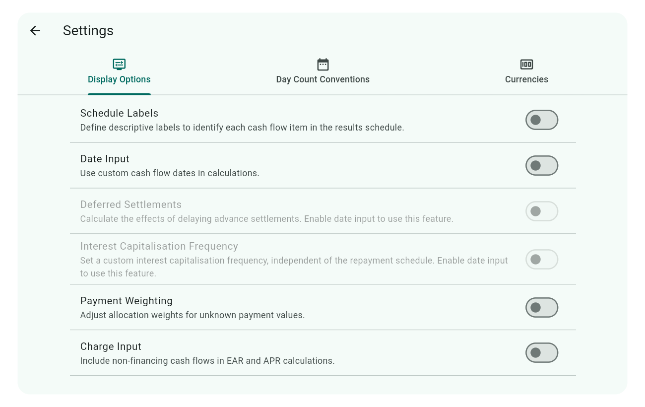
Here’s how the Display Options appear by default, with all options disabled, catering to simple financial calculations for everyday use:
For users with more complex needs, consider enabling the following features:
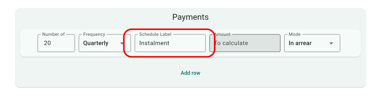
Schedule Labels
Enable this feature to add descriptive labels to each row under Advances, Payments, or Charges in the calculator input screen.
These labels appear in the results schedules, providing context for each entry.
Tip
Use singular forms for labels like “Rental” instead of “Rentals” for clarity in individual row descriptions.
Date Input
Activate this feature to manually set custom cash flow dates for your calculations. Once activated, the date input fields replace the Mode dropdowns in the calculator input, and the dates entered mark the start of each series.
Note
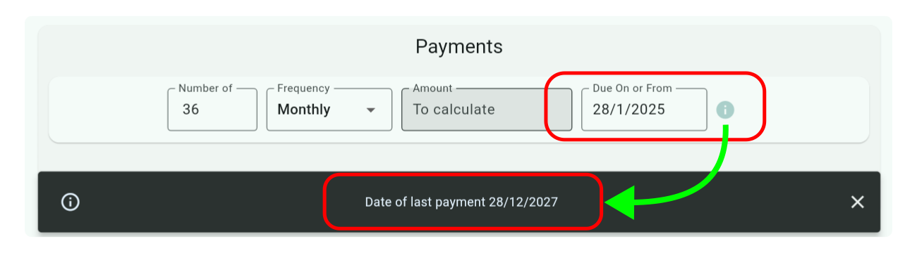
An information icon next to date fields in the Payments section provides additional context. Tapping this icon will display a snackbar at the bottom of the screen, revealing the date of the last payment in the series. This is crucial for constructing complex payment schedules.
For Detailed Usage: Explore examples 07, 09, 10, 12, 13, 14, and 15 for a thorough understanding of how to apply date inputs in various scenarios.
Important
Calculations always use dates, whether this feature is enabled or not. If disabled, the calculator uses dates from your device/system; when enabled, it uses the dates you specify. Thus, result schedules will always display dates, unaffected by this setting.
Deferred Settlements
Activate this feature to explore how delaying payments from a lender to an equipment supplier affects financial calculations under a finance contract. This vividly illustrates the concept of the time value of money and is particularly useful for lenders, though informative for all users.
Note: Enabling date input is required for this feature to function.
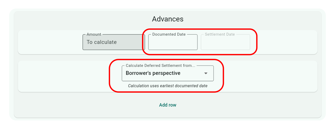
When activated, each row in the Advances section will feature two date fields:
Documented Date: This is the start date of the finance contract from the borrower’s viewpoint or the date of subsequent drawdowns if there are multiple advances before settlement.
Settlement Date: This date, which is on or after the Documented Date, marks when the supplier receives payment, hence the term ‘deferred settlement.’
A dropdown menu also appears, allowing you to choose the perspective for calculations:
Borrower’s Perspective - Using the earliest Documented Date.
Lender’s Perspective - Using the earliest Settlement Date.
For In-Depth Exploration: Check out examples 13, 14, and 15 to gain a comprehensive understanding of this feature’s application and benefits.
Interest Capitalisation Frequency
Activate this setting to customise how often interest is capitalised, independently from the repayment schedule. You must enable date input to use this feature.
Input Configuration:
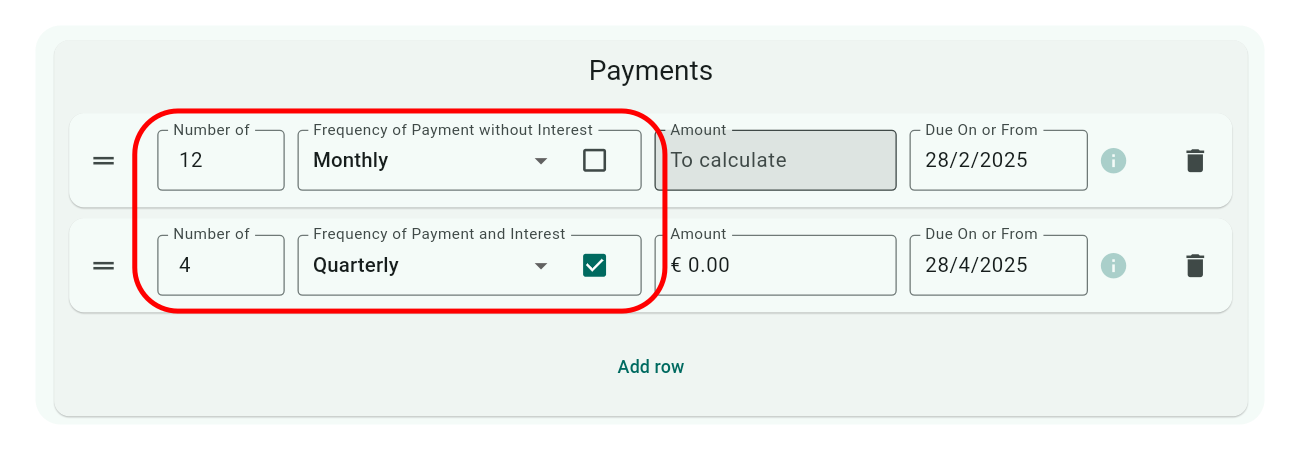
Create at least two rows in the Payments section:
For regular payments, uncheck the interest checkbox next to the frequency dropdown.
For interest capitalisation, check the interest checkbox and set the amount to zero to avoid unexpected results.
Example: The screenshots above and below show a scenario with monthly repayments and quarterly interest capitalisation. Note how every three months, the interest and repayment schedules align.
Detailed Example: For a deeper dive, see example 07.
Important
Ensure both the payment and interest schedules conclude on the same date for accurate calculations. Use the information icon next to date fields to confirm the longest dated end points of both schedules match.
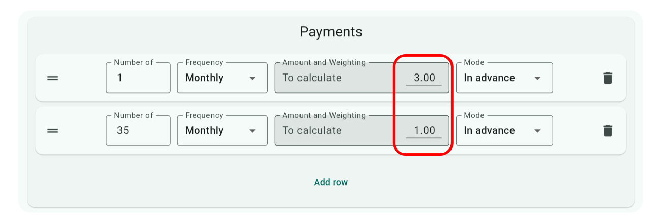
Payment Weighting
Activate this setting to allocate weights to unknown payment values when dealing with calculations involving two or more payment series rows. An additional input field appears next to the amount field for setting the weighting of the unknown value.
This feature allows for proportional distribution of an unknown payment across multiple series, rather than solving for a single value.
For In-Depth Exploration: Check out examples 05 and 08 to explore this feature’s potential.
Notes:
Single Series Effect: Applying a weight to a single payment series does not alter the result; the entire unknown value is assigned to that series.
Known Payments: If a payment value is known, a weighting of 1 is automatically applied and cannot be changed.
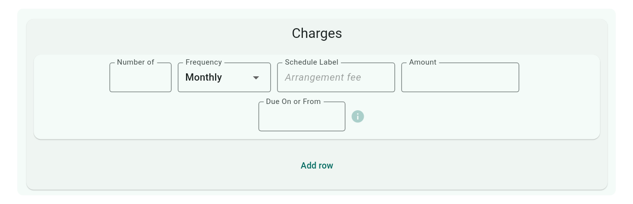
Charge Input
Enable this setting to include non-financing cash flows in calculations. A Charges section appears on the input screen when activated.
Curo Calculator can solve for unknown interest rates or cash flow values, taking these defined charges into account. This is particularly useful for calculating legally mandated APR interest rates, which must include all mandatory charges associated with consumer credit agreements.
Each charge series row includes a Payment Method drop-down menu, allowing you to specify whether the charge is Cash-paid (paid directly by the borrower) or Financed (financed and added to the loan principal). This selection determines whether the charge is included in calculations, depending on the chosen Day Count Convention:
Standard Conventions (e.g., 30/360, Actual/Actual): Cash-paid charges are excluded as they do not affect the financed amount, while Financed charges are included as they increase the principal.
APR/EAR Conventions (e.g., US Appendix J APR, EU 2023/2225 APR): Cash-paid charges are included as they impact the total borrowing cost, while financed charges are excluded as they are assumed to be part of the provided rate or cash flows.
The table below summarizes how charges are handled based on the day count convention:
Day Count Convention Type
Cash-paid Charge Included?
Financed Charge Included?
Standard Conventions
No
Yes
APR/EAR Conventions
Yes
No
In the screenshot, both Label and Date inputs have been activated in Settings. For calculations involving charges, enabling Date Input is advisable to account for one-off charges at the end of the finance term.
For Detailed Usage: Explore example 18 to see how charges are applied in APR calculations.
Tip
Use the Payment Method drop-down to accurately model charges for regulatory compliance, such as including Cash-paid charges in US Appendix J APR, EU 2023/2225 APR, or other APR calculations.
Day Count Conventions
Note
This section describes how to manage day count conventions used in calculations. For a deeper understanding of what day count conventions are and their significance, visit Core Concepts > Day Count Conventions.
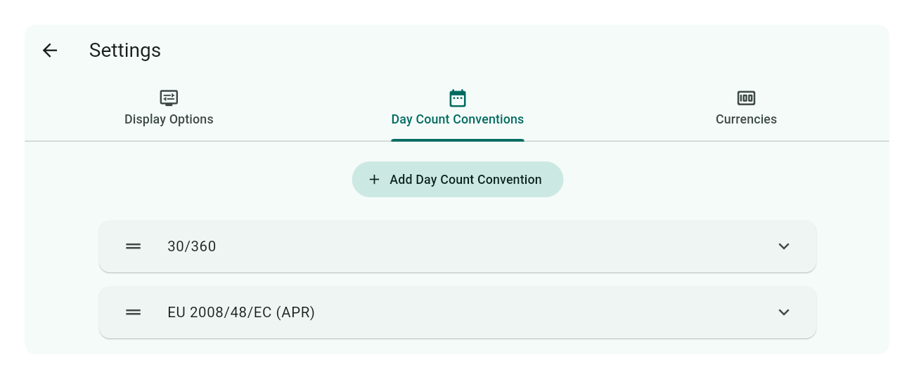
Upon app installation, a number of day count conventions are automatically added. These appear in an orderable list as shown below:
To reorder conventions, simply press and hold the drag and drop icon on the left of each convention row, then drag it to your preferred position.
The first convention in the list is set as the default and will be the first option in the Day Count Convention dropdown menu at the bottom of the calculator’s input screen, just above the Calculate button, as shown here:
Since all conventions are predefined and not user-modifiable, your options are limited to adding or deleting conventions from the list.
Add a Day Count Convention
Click or tap the Add Day Count Convention button above the convention list. This action will open a scrollable selector panel displaying available conventions not yet selected, each accompanied by a description of how the duration between cash flows is calculated. Choosing a convention dismisses the pop-up and adds your selection to the end of the list.
Delete a Day Count Convention
To remove a convention, click or tap the row of the Day Count Convention you wish to delete. The panel will expand, revealing a delete icon at the bottom right corner. Click this icon to remove the convention from the list. If you later need the convention, you can simply add it back as described above.
Note
You cannot delete the last remaining convention; there must always be at least one selected.
Currencies
Note
As explained elsewhere in this guide, the currency settings primarily affect how monetary data is displayed. However, the decimal precision set for each currency does influence calculations. Despite this, switching between currencies does not alter the nominal input values of the calculations.
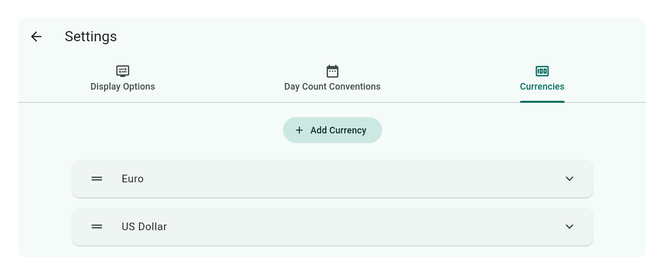
Upon app installation, a number of example currencies are automatically added. These are displayed in an orderable list as shown below:
The first currency listed is set as the default for display purposes. To reorder currencies, simply press and hold the drag and drop icon on the left of each currency row, then drag it to your preferred position.
All defined currencies will appear in the currency selector on the calculator’s input screen. To access this selector, click or tap the money icon at the top right corner of the input screen, as indicated here:
The next section will guide you on how to add, modify, or delete currencies.
Add a Currency
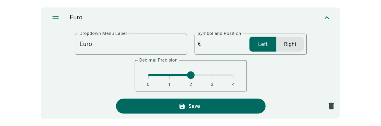
Click or tap the Add Currency button above the currency list. A new input panel will appear below the last currency:
Input Actions:
Dropdown Menu Label: Enter a short, unique title for the currency, which will appear in the currency selector. This field is required.
Symbol and Position: Specify your currency symbol and use the switch to decide if it should appear on the left or right of monetary values. This field is optional; leave blank for uncluttered display.
Decimal Precision: Use the slider to set the number of decimal places (0 to 4) for financial calculations, affecting both input and result displays. While typically you’d use the standard precision for the currency, you’re free to choose otherwise.
Once done, click or tap Save.
Edit a Currency
To modify a currency, tap on its row to open the input panel. Make your changes and then click or tap Save.
Delete a Currency
To remove a currency, tap on its row to expand the input panel, then select the delete icon. You’ll be prompted with a confirmation dialog to proceed.
Note
You cannot delete the last remaining currency; there must always be at least one defined.
My Templates
Templates simplify repetitive calculations with similar inputs. Curo Calculator leverages templates to provide numerous examples, guiding you through its features. You can modify any example, tailoring it to your needs, and save it as a personal template, avoiding the hassle of starting from zero. With just a few clicks or taps, execute your tailored calculations, making this one of the most user-friendly yet powerful tools available!
Start streamlining your calculations today with Curo Calculator Templates!
Subsections of My Templates
Creating a Template
You have two options for creating templates, each with its own benefits and drawbacks:
Create a Template from Scratch: This approach offers more flexibility, but requires you to manually adjust the calculator’s display options to activate the features you need.
Create a Template from a Calculator Example: This is by far the quickest and easiest method, but you cannot modify the display options of the loaded example.
Important
When a Calculator Example or a Template you’ve created is loaded, the Settings > Display Options used in its creation are applied and cannot be modified afterward. Therefore, creating a Template from an Example might not always be the best approach.
Regardless of the method you choose, the first step is to enter or modify all required calculation inputs. Perform a calculation to verify your inputs are correct for templating. Adjust and repeat as necessary. Once satisfied with the results, proceed to save these inputs as a Template.
Saving a Template
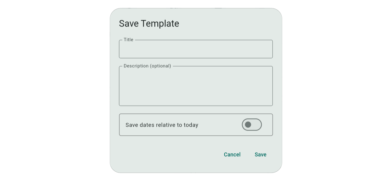
At the top of the calculator input screen, select the Save Icon as shown in the image.
This will launch a pop-up window as shown in the image. Field descriptions are provided below.
Title: The title should uniquely identify your template for ease in identification and selection from a list of potentially many templates.
Description: The description, which is optional, provides additional context beyond what the title suggests.
Save Dates (switch): This switch is only displayed when a template contains date inputs. The two date-save options are:
Save dates relative to today (button off): All dates are preserved as offsets from the current device/system date. When a template is loaded in the future, dates are rebased on the device/system date at that time, with offsets reapplied.
Save dates as entered (button on): All dates are preserved exactly as entered.
Select the Save button when you’ve finished, or the Cancel button to abort. A snackbar at the bottom of the screen will confirm once the template has been saved.
After creating one or more templates, you’ll need to explore Managing Templates, a topic covered next.
Managing Templates
To access the screen for managing templates, first tap or click the three-bar icon in the top left corner of the app. This action will display a sidebar menu. From there, select My Templates to load the management screen.
The scope for managing templates is limited to amending the Title and Description provided at the time of creating a template, deleting a template, and assigning a template to load on app startup (all described below).
Note
You cannot amend the calculation template inputs and settings directly on this screen. To modify these, load the template you wish to change in the Calculator input screen, make your adjustments, and then re-save it as a Template. Return here to delete the old Template.
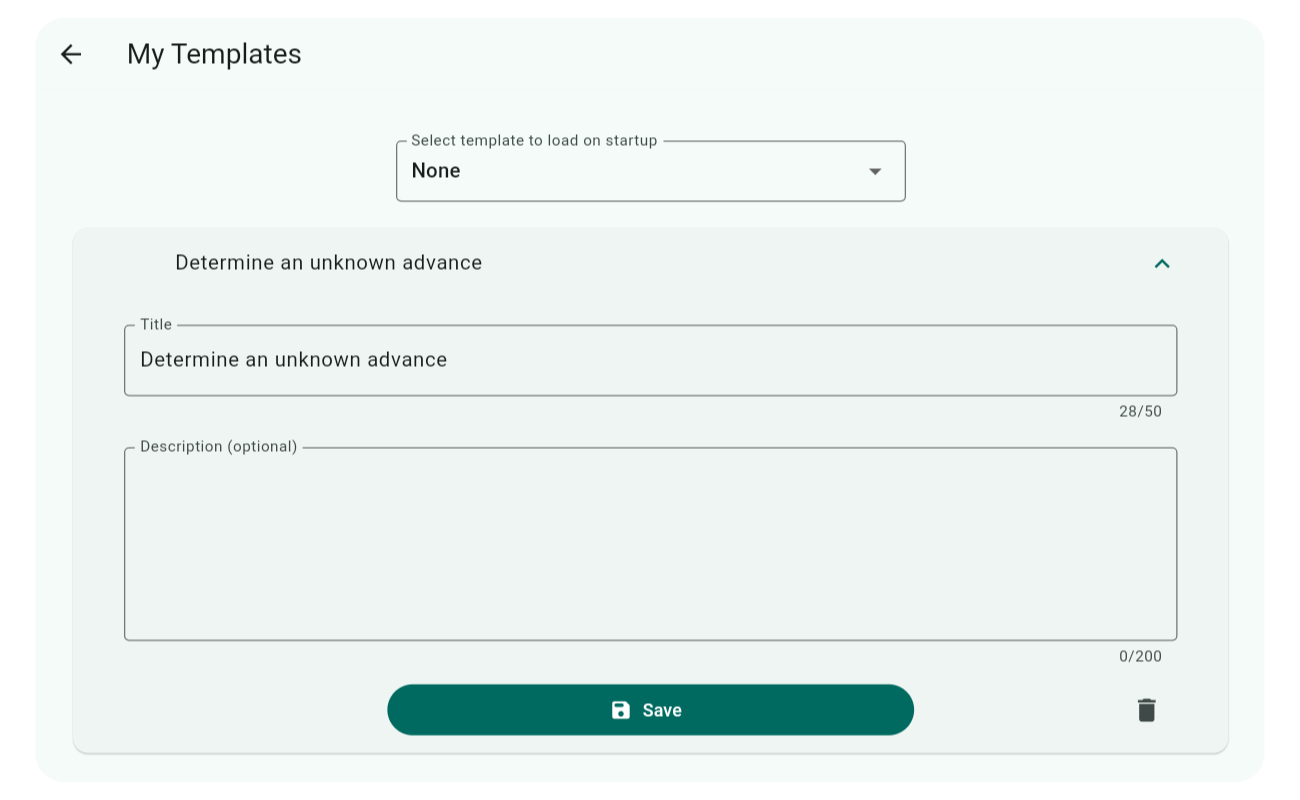
After creating your first template, the management screen will look something like the image below.
The first thing you’ll notice is the Select template to load on startup dropdown, located above the list of templates. This dropdown lists all your current templates, allowing you to designate a particular template to load at app startup. This option is particularly useful for Finance Professionals performing standard calculations daily rather than occasional users.
When you have more than one Template, a drag and drop icon appears on the left of each row, which you can use to reorder them. The ordering of templates is reflected in the Template pop-up selector accessed from the Calculator input screen.
Specific template actions include:
Edit: Tap the Template you wish to update in the list, and an expanding panel containing the Title and Description fields will appear. Make your changes and select Save.
Delete: Tap the Template you wish to delete, and in the expanding panel, select the Delete Trash icon. A confirmation dialog will pop up asking you to confirm the action.
Example Showcase
Curo Calculator comes equipped with numerous examples designed to guide you through the usage of its extensive features. These examples help you master specific calculations quickly, bypassing the need for a steep learning curve.
With just 3 clicks or taps, you can execute calculations ranging from simple to complex, making it one of the easiest tools to use!
Important
The examples use nominal cash flow values based on the Euro, which may not scale well across different currencies due to varying exchange rates. While you can set your preferred currency in the Settings > Currencies tab, these settings only affect how data is displayed; they do not alter the underlying calculation values. Therefore, when using a different currency, you might need to manually adjust the example values to better fit your local context.
To access the examples:
Look for the third button from the left on your panel of quick action buttons, as shown in the image below.
Tap or click this button to open a pop-up panel with a scrollable list of examples.
Select the example you’re interested in by tapping or clicking on it. This action will automatically configure the Display Options and fill the input screen with the example data.
To execute the calculation, simply press the ‘Calculate’ button.
Additional and more in-depth information on each example is available via the menu on the left. These examples are designed to complement the calculation inputs by providing contextual insights into how the calculations work. They extensively use diagrams to visually explain financial cash flows, which is covered next.
Cash Flow Diagrams
A cash flow diagram is a visual tool that represents the timing and direction of financial transactions in a straightforward manner. The diagram below is taken from Example 1, typical of the diagrams accompanying other examples.
Understanding the Diagram:
Time Line: The diagram starts with a horizontal line representing the duration or contract term, which is typically divided into compounding periods.
Cash Flow Arrows:
Upward Arrows signify cash inflows, such as money received by the lender, marked at the point on the timeline where the transaction happens.
Downward Arrows indicate cash outflows, or money paid out by the lender.
Relating to the Calculator:
The down arrow cash flows correlate with the data you input in the Advances section of the calculator input screen.
Conversely, up arrow cash flows correspond to entries in the Payments section, and if applicable, the Charges section (see Settings > Charge Input).
Note, we use coloured arrows to quickly identify the known and unknown values:
Red arrows are unknowns.
Blue arrows are knowns; if all arrows are blue, the interest rate is the unknown to solve.
There is one example with a green arrow, used to identify a non-financial charge cash flow.
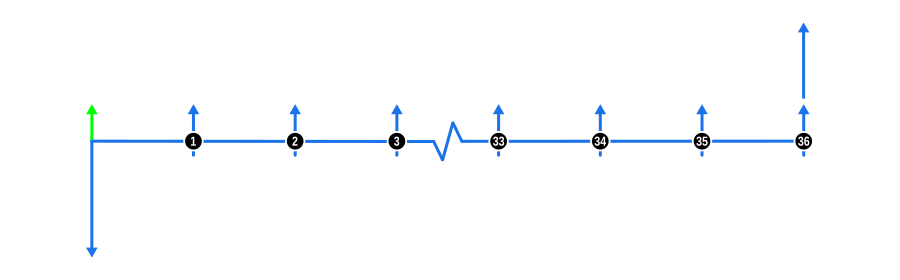
Where there are a series of identical values, we’ve condensed the timeline rather than displaying them all. A concertina line will be displayed at the appropriate point, and we’ve numbered the payment cash flows before and after that point so you don’t lose track of the totals.
This visual representation helps in understanding how each transaction impacts the overall financial scenario over time, making complex calculations more intuitive.
Subsections of Example Showcase
Example 1
Determine an advance amount
This example shows how to determine the maximum loan amount you can afford for personal or business needs. It calculates this based on your regular payment capacity and the lender’s interest rate.
This example illustrates the concept of discounting future cash flows to determine their present value, which is crucial for assessing loan affordability. The diagram below visualises the cash flow dynamics:
Example Calculation Inputs
Advance: This is shown by a red downward arrow at the start of the timeline, indicating the amount you’re solving for.
Payments: Represented by blue upward arrows, these are the regular payments you can manage.
Interest Rate: Although not shown in the diagram, this rate is used to discount the future payments to their present value. It can be based on a best guess or actual lender rate.
Benefits and Implications
Understanding how much you can borrow is vital for making informed financial decisions, especially when considering purchasing significant items. If the calculated loan amount falls short of what you need:
You might need to contribute additional funds.
Extend the loan term to lower monthly payments.
Seek a lender with more favourable rates.
If the calculated amount exceeds your requirements:
You could opt for lower monthly payments.
Shorten the loan term to reduce overall interest paid.
This example helps you navigate these decisions by providing a clear financial picture based on your current capacity and market rates.
Example 2
Determine the deposit required
This example shows how to calculate the smallest deposit required for an asset purchase, using your regular payments and the lender’s interest rate.
This example illustrates how to determine the contribution required when the value of discounted future cash flows falls short of the full cost of an item. The diagram below visualises the cash flow dynamics:
Example Calculation Inputs
Advance: This is shown by a blue downward arrow at the start of the timeline, indicating the full cash price or loan value before your contribution is known.
Payments:
The red up arrow at the start of the time line is the deposit contribution you’re solving for.
Those represented by blue upward arrows are the regular payments you can manage.
Interest Rate: Although not shown in the diagram, this rate is used to discount the future payments to their present value. It can be based on a best guess or actual lender rate.
Benefits and Implications
Understanding how much you may be required to contribute towards the cost of an item is vital for making informed financial decisions, especially when considering purchasing significant items. If the calculated contribution amount exceeds the cash you have on hand:
Extend the loan term to lower the contribution payment.
Seek a lender with more favourable rates.
If the calculated amount is lower than what you may wish to contribute:
You could opt for lower monthly payments.
Shorten the loan term to reduce overall interest paid.
This example helps you navigate these decisions by providing a clear financial picture based on your current cash resources and market rates.
Example 3
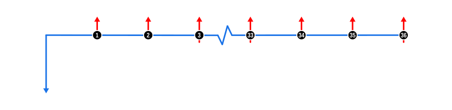
Determine a payment in an arrears repayment profile
This example demonstrates how to calculate the value of a payment when it’s due at the end of each repayment period, known as ‘in arrears’.
This example illustrates the use of one of two Modes, a core concept in financial calculations, when solving for unknowns. To mix things up, the ‘In arrear’ payments are assigned a quarterly frequency. The diagram below visualises the cash flow dynamics:
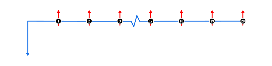
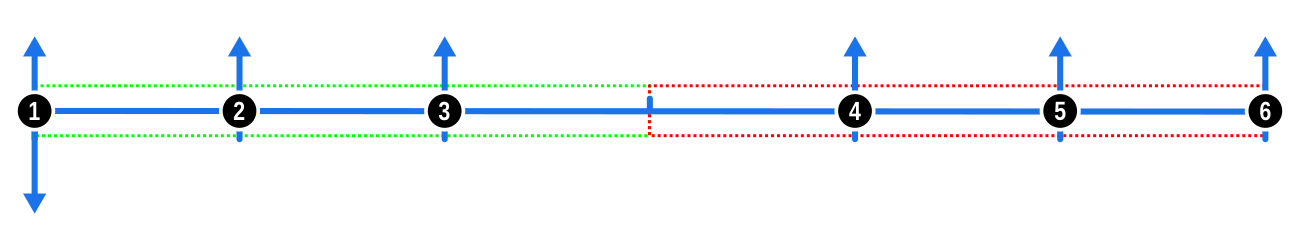
Example Calculation Inputs
Advance: This is shown by a blue downward arrow at the start of the timeline, indicating the value is known.
Payments: Represented by red upward arrows, these are the regular quarterly payments. Notice how the first payment in the series occurs at the end of the first quarter after the Advance, and the remaining payments regularly thereafter.
Benefits and Implications
Understanding the impact Modes can have in calculations is important for these reasons:
Payments ‘In arrear’ increase the overall interest repaid as capital reduction is delayed (as opposed to ‘In Advance’ covered in example 4).
As a borrower, knowing the mode used in finance quotes allows for accurate comparison; for instance, the implicit rate in a given repayment profile containing the same payment amount can vary significantly based on the repayment Mode, although the gap in the implicit rates tends to narrow as repayment terms lengthen.
Cash Flow Management: ‘In arrear’ payments can align better with certain cash flow cycles, such as receiving income at the end of a period, which might be more suitable for managing personal or business finances.
Impact on Total Interest: Understanding how ‘in arrears’ payments affect the total interest paid over the life of a loan can influence decisions on loan terms, especially for longer-term loans where the difference in interest can be substantial.
Negotiation Power: Knowledge of payment modes can provide leverage when negotiating loan terms with lenders, potentially leading to better rates or terms if you can argue for a mode that suits your financial planning.
Budgeting: For budgeting purposes, ‘in arrears’ payments allow for one more period of interest accumulation before the first payment, which might require adjustments in short-term financial planning.
Loan Products: Some loan products, like certain mortgages or business loans, might only offer ‘in arrears’ payment structures, so understanding this mode is crucial for those considering these financial products.
This example helps you navigate these decisions by providing a clear financial picture based on different repayment structures and their implications on your financial health.
Example 4
Determine a payment in an advance repayment profile
This example demonstrates how to calculate the value of a payment when it’s due at the beginning of each repayment period, known as ‘in advance’.
This example illustrates the use of one of two Modes, a core concept in financial calculations, when solving for unknowns. The ‘In advance’ payments are assigned a monthly frequency to show contrast with the previous example. The diagram below visualises the cash flow dynamics:
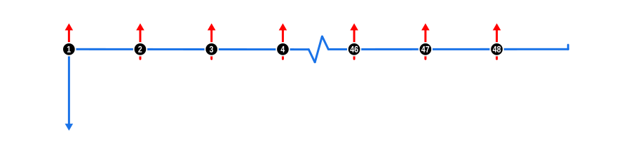
Example Calculation Inputs
Advance: This is shown by a blue downward arrow at the start of the timeline, indicating the value is known.
Payments: Represented by red upward arrows, these are the regular monthly payments. Notice how the first payment in the series occurs at the start of the first month coinciding with the Advance, and the remaining payments regularly thereafter.
Benefits and Implications
Understanding the implications of ‘In advance’ payment modes in financial calculations is crucial for these reasons:
Payments ‘In advance’ reduce the overall interest repaid since capital reduction starts immediately (as opposed to ‘In arrears’ in Example 3).
As a borrower or investor, recognising the mode helps in comparing financial products more accurately; for example, the effective interest rate can be lower with ‘in advance’ payments due to quicker principal reduction.
Cash Flow Management: ‘In advance’ payments might require more initial cash on hand but can lead to lower total interest costs, beneficial for those with sufficient cash reserves.
Savings on Interest: Over the life of the loan, ‘in advance’ can result in significant savings on interest, especially for long-term loans or high-interest scenarios.
Budget Planning: This mode can affect monthly budgeting, as payments are due from the outset, which might be challenging for those with irregular income patterns.
Negotiation: Understanding ‘in advance’ can give you an edge in loan term negotiations, possibly securing lower rates or better terms due to the lender’s reduced risk exposure.
Loan Comparison: When comparing different loan offers, knowing if payments are ‘in advance’ or ‘in arrears’ can significantly alter the perceived cost of borrowing.
Investment Products: For investments or annuities that pay ‘in advance’, the timing can affect the calculation of return rates, making it advantageous for investors looking for immediate income streams.
This example aids in understanding how payment timing affects financial outcomes, enabling better decision-making in personal or business finance scenarios.
Example 5
Determine a payment in a 3+33 repayment profile
This example demonstrates how to calculate a payment schedule where the first three payments are due at the contract’s start, known as ‘in advance’. The remaining payments are then spread out. This structure is commonly utilised in small business loans, particularly for leasing arrangements.
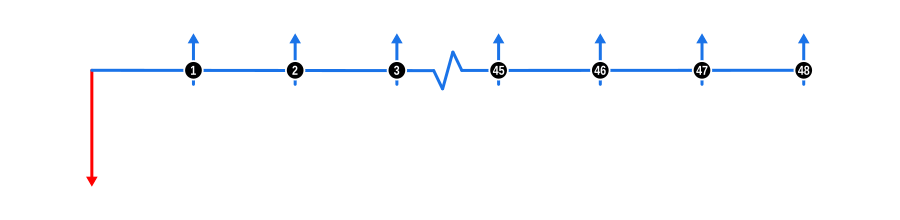
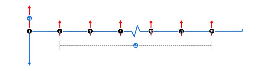
This example illustrates the use of ‘front loading’ a repayment profile on a proportional basis when solving for unknowns, and makes use of the Payment Weighting calculator feature. The 3+33 repayment structure is common in small business leasing arrangements, and variations on this exist, such as 3+35. This example is designed specifically for Finance Professionals, though it should be informative for all users. The diagram below visualises the cash flow dynamics:
Example Calculation Inputs
Advance: This is shown by a blue downward arrow at the start of the timeline, indicating the value is known.
Payments: Represented by red upward arrows, these are the regular payments. Notice though how the first payment in the series coincides with the Advance and is annotated with the x3 annotation. This is the weighted payment, followed by the remaining payments regularly spaced. The timeline continues for a further month after the final payment, suggesting the contract ends at the end of the final payment period. Note however the contract end date may vary between lenders and may also depend on the number of payments taken in advance.
Tip: It is permissible to assign whatever weighting ratio you need to the unknown values of two or more payment rows.
Benefits and Implications
The front loading of a repayment profile is typically used for these reasons:
Risk Reduction: By securing multiple payments upfront, lenders reduce their risk exposure, especially in cases where there’s a higher likelihood of default early in the loan term.
Cash Flow Management for Lenders: This structure provides immediate cash flow to the lender, which can be critical for managing liquidity, especially for smaller lending institutions or during economic downturns.
Encouraging Loan Commitment: Front-loaded payments can incentivise borrowers to commit more seriously to the loan terms, knowing they’ve already made substantial payments at the outset.
Adjusting for Seasonality: In industries with seasonal income, a 3+33 structure might align better with the financial cycle, allowing for lower payments during off-peak times while capitalising on peak cash flows initially.
Tax Benefits: For the borrower, this structure might offer tax advantages if the payments are deductible, and making larger payments earlier in the fiscal year can maximise this benefit.
Tailoring to Client Needs: Lenders can use this feature to customise loan terms to match the cash flow profile of different businesses, offering flexibility in how much is paid upfront versus over time.
Pricing Strategy: The 3+33 profile might allow for different pricing strategies, where the interest rate or total cost of borrowing might be adjusted based on the reduced risk from front-loaded payments.
Lease vs. Purchase Decisions: In leasing scenarios, this structure can make the lease more attractive by reducing the upfront cost while still providing the lender with security through immediate payments.
This example helps finance professionals understand how to leverage payment weighting to structure loans that balance risk, cash flow, and client satisfaction in various financial contexts.
Example 6
Determine a payment with a balloon payment included
This example shows how to calculate a payment schedule that includes a significant final payment, known as a ‘balloon payment’. This amount might also be called a ‘future value’ or ‘guaranteed minimum future value’, depending on whether it’s for a loan or lease.
This example illustrates how to determine the payment value in a repayment schedule which incorporates a balloon or future value at the end of a repayment term. The diagram below visualises the cash flow dynamics:
Example Calculation Inputs
Advance: This is shown by a blue downward arrow at the start of the timeline, indicating the value is known.
Payments: Represented by red upward arrows, these are the regular unknown payments. Coinciding with the final payment is a larger blue up arrow representing the known balloon payment.
Benefits and Implications
Balloon payments are commonly utilised in various financial arrangements, particularly in:
Asset Financing:
Vehicles and Equipment: Often used in car loans or equipment financing where the lender anticipates a significant residual value at the end of the term. This can be structured as an operating lease where the lender guarantees the value of the asset at lease end.
Benefits for Borrowers: Allows for lower monthly payments, making high-cost purchases more manageable within cash flow constraints. It might also align with expectations of selling or refinancing the asset at the end of the term.
Risks for Borrowers: Requires planning for a large lump sum payment or refinancing at the end, which could be challenging if financial conditions change.
Business Loans:
Small Business: Balloon payments can be part of business loans where the business expects significant revenue or an event like selling the business at the end of the loan term.
Strategic Financial Planning: Businesses might use balloon payments to match their cash flow cycles, expecting to pay off the loan with proceeds from future business success.
Lenders’ Perspective:
Risk Management: By structuring a loan with a balloon payment, lenders can manage risk by ensuring a significant portion of the loan is repaid at the end, potentially secured by the asset’s residual value.
Lease Rentals: In leases, balloon payments help in calculating rentals that account for the asset’s expected future value, providing a balance between regular payments and end-term value.
Investment and Savings:
Structured Savings Plans: Certain savings or investment plans might use balloon payments to encourage long-term saving or investment, with the balloon representing a maturity or payout amount.
Market Conditions:
Economic Cycles: In fluctuating markets, balloon structures can be adjusted to match economic forecasts, providing flexibility in repayment during uncertain times.
Understanding the dynamics of balloon payments is essential for both borrowers and lenders to manage cash flows, plan for future financial obligations, and structure agreements that align with anticipated asset values or business performance. This example provides a foundation for users to understand and navigate these financial structures effectively.
Example 7
Determine a payment using a different interest frequency
This example demonstrates how to calculate a payment when interest is compounded at one frequency, separate from the payment schedule. This setup is common in consumer loans, like those with monthly repayments and quarterly interest compounding. Be mindful when performing these types of calculations that both the payment schedule and interest schedule should end on the same date to maintain consistency.
This example illustrates how to determine the payment value in a repayment schedule with a separate compounding frequency, in this case monthly repayments with quarterly interest. This example demonstrates the Interest Capitalisation Frequency feature of the calculator and is designed specifically for use by Finance Professionals, though it should be informative for all users. The diagram below visualises the cash flow dynamics:
Example Calculation Inputs
Advance: This is shown by a blue downward arrow at the start of the timeline, indicating the value is known.
Payments:
The regular unknown payments are represented by red upward arrows.
The quarterly interest capitalisation payments cannot be displayed as they have a zero value. However, there is one cash flow diagram notation used in this guide which has not been discussed yet, and that is the payment up arrows also extend for a short distance below the timeline. We use this to signify the payment includes capitalised interest. Note therefore in this example that the line only extends every third payment, when the repayment and interest schedules align.
Benefits and Implications
These types of repayment schedules are often found in consumer products offered by high street banks, with the following benefits and considerations:
Alignment with Accounting Practices:
Simplified Accounting: By aligning interest compounding with accounting cycles (like quarterly reports), it can simplify the tracking and reporting of interest income for banks.
Financial Reporting: Easier to match interest income with the periods in which it is earned, which is crucial for accurate financial statements.
Interest Rate Management:
Rate Adjustment: Allows for more frequent adjustments in interest rates based on market conditions if compounded more often than payments are made, potentially benefiting lenders during rising rate environments.
Consumer Loan Products:
Product Flexibility: Can be marketed as offering lower monthly payments while still providing the bank with higher effective interest rates due to compounding.
Borrower Perception: Monthly payments might seem more manageable to borrowers, potentially increasing loan uptake despite higher effective interest.
Risk Management:
Interest Capitalisation: Compounding interest increases the amount of interest capitalised, thus increasing the total amount owed more rapidly, which can act as a buffer for lenders against loan defaults.
Prepayment Penalties: Structures like this can lead to higher penalties for early loan repayment, protecting lenders’ expected interest income.
Regulatory Compliance:
Disclosure: This setup can affect how interest rates and total loan costs are disclosed to consumers, requiring clear communication to ensure compliance with financial regulations.
Liquidity Management:
Cash Flow Alignment: Might help banks manage liquidity by having a predictable schedule of interest income that doesn’t necessarily align with the outgoings for payments.
Product Differentiation:
Market Positioning: Can be used to differentiate loan products in a competitive market, offering unique repayment structures that cater to specific consumer segments.
Understanding these aspects can help finance professionals tailor loan products that not only meet consumer needs but also align with the strategic financial goals of lending institutions.
Example 8
Determine a payment using a weighted profile
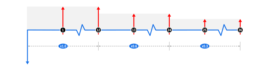
This example demonstrates how to calculate a payment schedule where early and mid-term payments focus on reducing the principal faster. This method is often adopted in small business loans to align with asset depreciation rates.
This example illustrates solving unknown payments on a proportional basis to accelerate capital repayment using a stepped profile. It makes use of the Payment Weighting calculator feature and is designed specifically for Finance Professionals, though it should be informative for all users. The diagram below visualises the cash flow dynamics:
Example Calculation Inputs
Advance: This is shown by a blue downward arrow at the start of the timeline, indicating the value is known.
Payments: The regular unknown payments are represented by red upward arrows. As the example uses three 12 monthly payment series with assigned weightings of 1.00, 0.60, and 0.30 respectively, we’ve adjusted the height of the upward arrows to reflect the reduction in payment values over time, and have also used a light grey background to emphasise the stepped profile.
Benefits and Implications
These types of repayment schedules are often found in business lending, with the following benefits and considerations:
Accelerated Principal Reduction:
Risk Mitigation for Lenders: By front-loading payments, the principal is reduced more quickly, thereby lowering the lender’s exposure to credit risk over time.
Interest Savings for Borrowers: Paying down the principal faster reduces the total interest paid over the life of the loan, benefiting the borrower financially.
Alignment with Business Cycles:
Cash Flow Management: This structure can be tailored to match expected business income, where higher payments are feasible during peak revenue periods, and lower payments during slower times.
Depreciation Matching: For assets that depreciate more rapidly in the early years, this payment structure can align repayments with the asset’s useful life, improving financial reporting and tax planning.
Incentivising Borrower Performance:
Performance-Based Repayments: Can be structured to reward early success or growth in business by allowing for lower payments if certain performance metrics are met.
Flexibility in Loan Structuring:
Customisation: Lenders can customise loan terms to better fit the financial trajectory of the borrowing business, potentially attracting clients with bespoke financial solutions.
Negotiation Leverage: Offers a negotiation point where both parties can discuss how the payment schedule reflects actual or projected cash flows.
Regulatory and Compliance:
Transparency: Must be clearly communicated to avoid misunderstandings about payment obligations, which is crucial for maintaining trust and compliance with lending regulations.
Market Differentiation:
Competitive Edge: Lenders offering stepped payment profiles can differentiate themselves in the market, appealing to businesses looking for repayment plans that adapt to their growth patterns.
Loan Portfolio Management:
Diversification: Allows lenders to diversify their loan portfolio with varied repayment structures, potentially spreading risk across different types of loan products.
Encouraging Financial Discipline:
Discipline in Borrowing: Encourages businesses to manage their finances more stringently in the early stages of the loan, fostering a culture of financial discipline.
This stepped payment approach provides a strategic tool for both lenders and borrowers to manage financial obligations in a manner that supports business growth while minimising risk exposure for the lender. It’s a nuanced approach that requires careful consideration but can offer significant benefits when structured correctly.
Example 9
Determine a payment with periodic token payments
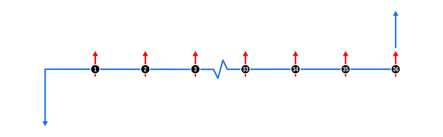
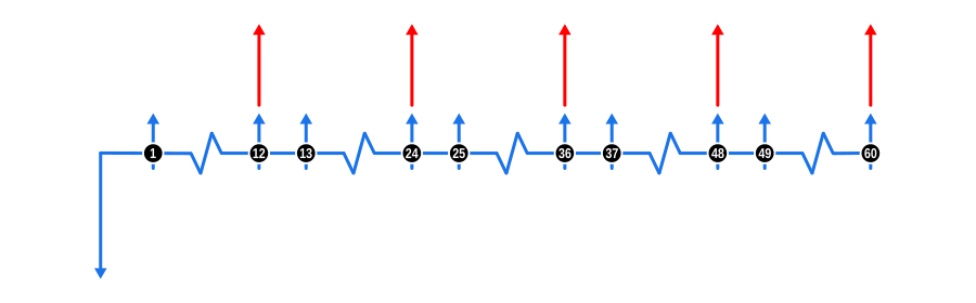
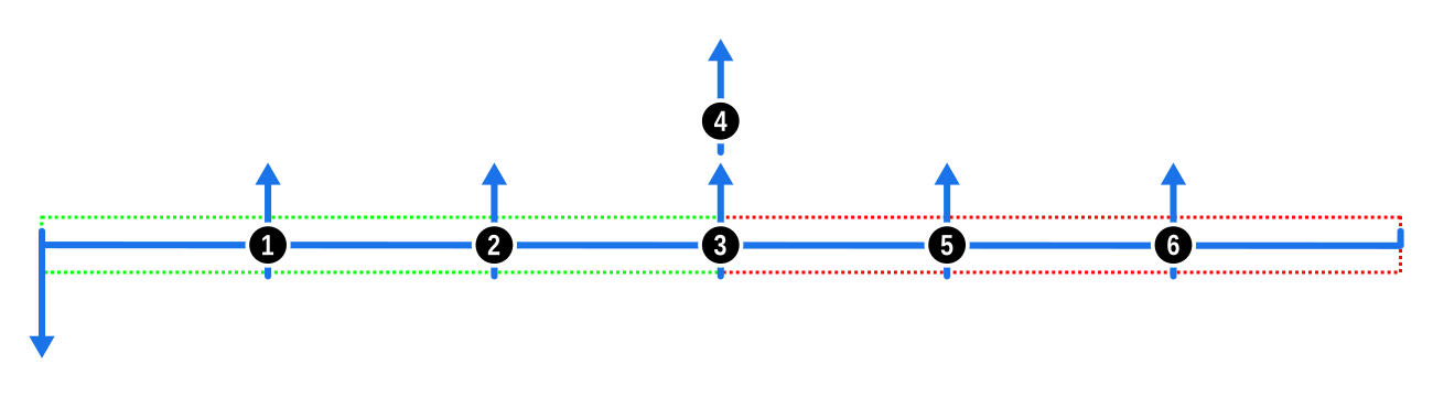
This example shows how to calculate a payment schedule with small, regular ’token’ payments and larger, less frequent payments, usually half-yearly or yearly. This structure is common in agricultural lending, where payments match seasonal income, and the token payments help prevent interest from compounding.
This example illustrates how to incorporate frequent token or contact payments into a repayment structure that has larger, less frequent repayments. It is designed specifically for Finance Professionals, though it should be informative for all users. The diagram below visualises the cash flow dynamics:
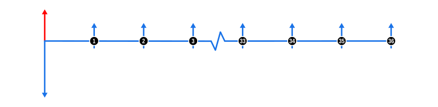
Example Calculation Inputs
Advance: This is shown by a blue downward arrow at the start of the timeline, indicating the value is known.
Payments: The frequent monthly contact payments are represented by blue upward arrows, and the larger, less frequent annual payments are represented by red upward arrows. Note that each annual payment coincides with the 12th consecutive contact payment, so in practice, these are lumped together as a single payment.
Benefits and Implications
This payment structure is particularly beneficial in scenarios where cash flows are seasonal or irregular:
Seasonal Income Alignment:
Agricultural and Seasonal Businesses: Matches repayment with harvest or sales seasons, ensuring payments are made when income is highest.
Cash Flow Management: Small token payments keep the loan from defaulting or accruing excessive interest during low-income periods, while larger payments clear substantial portions of the principal when funds are available.
Interest Management:
Reducing Compounding Interest: Token payments serve to partially pay down interest, reducing the amount of interest that compounds over time, thus saving on total interest costs.
Risk Mitigation for Lenders:
Consistency: Regular small payments provide a steady, albeit minor, cash flow, reducing some risk of default by keeping the loan active.
Security: Larger periodic payments act as checkpoints to ensure the loan remains on track, providing security against the risk of non-payment over longer intervals.
Borrower Flexibility:
Budgeting: Helps in budgeting for both borrowers and lenders, as small payments are predictable and manageable, with the larger payments planned around anticipated income spikes.
Encouraging Loan Commitment:
Engagement: Frequent small payments can psychologically commit the borrower more to the loan, reducing the likelihood of default.
Tax and Financial Planning:
Deductions: For borrowers, regular payments might offer more consistent tax deductions, while the larger payments can be planned around fiscal year ends for tax advantages.
Customisation for Borrower Needs:
Tailored Solutions: Lenders can offer this structure to cater specifically to industries or clients with known seasonal cash flow patterns, enhancing customer satisfaction and loyalty.
Market Expansion:
Market Fit: This structure can open up lending to sectors traditionally seen as high risk due to their income cycles, by adapting the repayment schedule to their financial rhythm.
Regulatory and Compliance:
Transparency: Ensures clarity in loan agreements, detailing when and how much will be paid, aiding in compliance with consumer protection laws.
Implementing such a repayment structure requires careful planning but can lead to a win-win situation where both lenders manage risk effectively, and borrowers manage their cash flows in alignment with their business cycles.
Example 10
Determine the supplier discount - 0% finance scheme
This example demonstrates how to calculate the supplier discount that offsets financing costs in 0% finance deals, often seen in vehicle purchases. If the terms between the supplier and lender are undisclosed, you’ll need to estimate the lender’s interest rate using current market rates to accurately determine this discount.
This example covers the topic of 0% and low-interest finance schemes from the perspective of a 0% finance lender. Examples 11 and 12 cover the same topic with slight variations from the perspective of a cash buyer seeking a discount, and a borrower wanting to use a 3rd party lender.
0% finance profiles can be characterised as containing disclosed and non-disclosed cash flows.
The disclosed cash flows, which a borrower is aware of, are the full retail cost (advance) of the financed item and the payment cash flows which contain principal only; the sum of payment cash flows equals the item cost (advance), hence 0% interest.
The non-disclosed cash flows are the direct transactions between supplier and lender, usually a cash discount to offset the financing costs of the lender.
This example, and the next two, should be informative for all users. The diagram below visualises the cash flow dynamics:
Example Calculation Inputs
Advance: The full retail cost of the financed goods is shown as a blue downward arrow at the start of the timeline.
Payments: The known borrower payments are represented by blue upward arrows. The supplier discount required to offset the financing costs is shown by a red upward arrow above the borrower’s upfront deposit at the start of the timeline.
Interest Rate: Although not shown in the diagram, the rate should reflect the return required by the lender.
Benefits and Implications
Mutual Benefits for Lender and Supplier:
New Lending Opportunities: For lenders, 0% finance deals are a way to expand their loan portfolio without directly charging interest to the borrower, instead getting compensated by the supplier.
Improved Stock Turnover: Suppliers benefit from quicker sales cycles as financing makes their products more attractive, reducing inventory holding costs.
Marketing Strategy:
Competitive Edge: Offering 0% finance can be a significant marketing tool for both parties, attracting customers who might not purchase otherwise due to cost concerns.
Cost Management:
Discount as Compensation: The supplier discount is essentially the cost of capital for the lender, which must be calculated to ensure the deal remains profitable for both parties.
Customer Acquisition:
Lower Barrier to Purchase: By removing interest costs, these deals lower the entry barrier for customers, potentially increasing sales volume.
Risk Management:
Credit Risk: Lenders might take on more risk since they’re not charging interest directly to the consumer, but they mitigate this through the discount from the supplier.
Supplier Risk: The supplier must ensure the discount doesn’t erode too much profit, balancing between sales volume and profit margin.
Market Dynamics:
Pricing Strategy: This model can influence market pricing, where suppliers might adjust their list prices knowing discounts will be given to offset financing.
Regulatory Considerations:
Disclosure: Both lenders and suppliers must navigate regulations regarding how such deals are advertised and disclosed to consumers to avoid misleading marketing.
Financial Planning:
Cash Flow: Suppliers need to plan for the immediate cash outflow due to discounts, while lenders must manage the timing of their cash inflows from repayments.
Consumer Perception:
Value Perception: The perception of getting “free” financing can lead to increased customer satisfaction and loyalty, even if the product’s list price might be adjusted to account for this.
This arrangement highlights a strategic partnership between suppliers and lenders, where careful calculation and transparency in undisclosed cash flows are crucial for maintaining a beneficial relationship while providing value to the end consumer.
Example 11
Determine the supplier discount required - cash versus 0% finance scheme
Building on Example 10, this example demonstrates how to calculate the minimum supplier discount needed to match the financial perks of a 0% finance scheme when paying with cash. Like before, you’ll have to estimate the lender’s interest rate for this calculation.
This example covers the topic of 0% and low-interest finance schemes from the perspective of a buyer wishing to secure the financial benefits associated with 0% finance when paying cash. Examples 10 and 12 cover the same topic with slight variations from the perspective of a 0% finance lender, and a borrower wanting to use a 3rd party lender.
This example, like the previous and the next, should be informative for all users.
As a cash buyer, it is important to understand how 0% finance works as it is from the analysis of the financial cash flows that the value of a potential cash discount can be derived and used as a starting point in supplier negotiations. The results and schedules produced by the calculator beyond that single discount figure are of little relevance, so can be safely ignored. With that covered, let’s move on!
0% finance profiles can be characterised as containing disclosed and non-disclosed cash flows.
The disclosed cash flows, which a borrower is aware of, are the full retail cost (advance) of the financed item and the payment cash flows which contain principal only; the sum of payment cash flows equals the item cost (advance), hence 0% interest.
The non-disclosed cash flows are the direct transactions between supplier and lender, usually a cash discount to offset the financing costs of the lender.
There is no need to be concerned about the non-disclosed cash flows; the calculation will use your best guess interest rate as a proxy to calculate this. How you obtain the disclosed cash flow information is simple. It is usually advertised by a supplier, and if it is not, request a finance quote… before you start talking discounts!
The diagram below visualises the cash flow dynamics for a hypothetical finance quote:
Example Calculation Inputs
Advance: The full retail cost of the goods (before discount) is shown as a blue downward arrow at the start of the timeline.
Payments: The quoted payments are represented by blue upward arrows. The supplier discount, derived by discounting these future payments, is shown by a red upward arrow at the start of the timeline.
Interest Rate: Although not shown in the diagram, the rate should reflect the market rate for a similar transaction. Sometimes this can only be based on guesswork, so perform a range of calculations to obtain a sense of what may be a good figure to aim for.
Benefits and Implications
For the Cash Buyer:
Negotiation Power: Understanding this calculation empowers cash buyers to negotiate discounts that effectively replicate the benefits of 0% financing.
Immediate Savings: The buyer gets the financial benefit upfront rather than over time, potentially improving cash flow management.
Avoidance of Financing Risks: By paying cash, buyers avoid any potential risks associated with financing, like changes in credit status or interest rates.
Simplified Purchase: No need to deal with loan documents, credit checks, or repayment schedules, simplifying the buying process.
For the Supplier:
Cash Flow Improvement: Immediate cash payment can improve the supplier’s cash flow, allowing for better inventory management or investment opportunities.
Supplier Not Losing Out: The discount given to the cash buyer is equivalent to what would have been given to the lender, maintaining the same profit margin.
Increased Sales Volume: Offering cash discounts can lead to more sales, especially if it matches or beats the appeal of 0% financing deals.
Reduced Administrative Costs: Less paperwork and administration associated with financing arrangements, potentially reducing operational costs.
Follow-on Opportunities: With the sale secured, suppliers can look forward to subsequent sales from maintenance, servicing, or related products, which are often more lucrative.
Market Positioning: Can position the supplier as flexible and customer-focused, appealing to buyers who prefer cash transactions or are wary of financing.
This approach demonstrates how understanding finance structures can lead to mutual benefits, where the cash buyer secures immediate financial benefits, and the supplier maintains profitability while potentially increasing customer satisfaction and future business opportunities.
Example 12
Determine the supplier discount required - own lender versus 0% finance scheme
Expanding on Example 10, this example shows how to calculate the minimum supplier discount necessary to equal the benefits of a 0% finance scheme if you opt for your own lender. Here, you can use your lender’s interest rate to ensure the discount leaves you financially neutral.
This example covers the topic of 0% and low-interest finance schemes from the perspective of a borrower wishing to secure the financial benefits associated with 0% finance when using own lender finance. Examples 10 and 11 cover the same topic with slight variations from the perspective of a 0% finance lender, and a cash buyer.
This example, like the previous two, should be informative for all users.
As with cash buyers, it is important for a borrower wanting to use their own lender facilities to understand how 0% finance works as it is from the analysis of the financial cash flows that the value of a potential cash discount can be derived and used as a starting point in supplier negotiations. Similarly, the results and schedules produced by the calculator beyond that single discount figure are of little relevance, so can be safely ignored. With that covered, let’s move on!
0% finance profiles can be characterised as containing disclosed and non-disclosed cash flows.
The disclosed cash flows, which a borrower is aware of, are the full retail cost (advance) of the financed item and the payment cash flows which contain principal only; the sum of payment cash flows equals the item cost (advance), hence 0% interest.
The non-disclosed cash flows are the direct transactions between supplier and lender, usually a cash discount to offset the financing costs of the lender.
There is no need to be concerned about the non-disclosed cash flows; the calculation will use your own lender interest rate as a proxy to calculate this. In this way, you can be assured the discount will leave you financially neutral. What this means is the total cost of finance using your own lender will be equal to or better than the total repayable under a 0% finance arrangement, provided the repayment profile remains unchanged. How you obtain the disclosed cash flow information is simple. It is usually advertised by a supplier, and if it is not, request a finance quote… before you start talking discounts!
The diagram below visualises the cash flow dynamics for a hypothetical finance quote:
Example Calculation Inputs
Advance: The full retail cost of the goods (before discount) is shown as a blue downward arrow at the start of the timeline.
Payments: The quoted payments are represented by blue upward arrows. The supplier discount, derived by discounting these future payments, is shown by a red upward arrow above the quoted upfront deposit at the start of the timeline.
Interest Rate: Although not shown in the diagram, the rate should reflect what your own lender has quoted.
Benefits and Implications
For the Own Lender Borrower:
Flexibility in Repayment Terms: Ability to negotiate different repayment terms with your own lender, which might offer better personal or business alignment than standard 0% finance terms (though this might alter the financial comparison).
Utilisation of Existing Credit: Make use of already approved credit lines, potentially avoiding additional credit checks or delays in securing finance.
Relationship Maintenance: Strengthen or maintain a good relationship with your existing lender, which can be beneficial for future financing needs.
Control Over Financing: Greater control over the financing process, including potentially lower interest rates or more favourable conditions than those offered in 0% schemes.
Customisation: Tailor the financing to match specific cash flow needs, potentially reducing overall interest costs if the loan term is adjusted accordingly.
For the Supplier:
Cash Flow Improvement: Receiving a cash discount from the supplier to the borrower’s lender can still improve the supplier’s cash flow similar to a cash deal.
Maintaining Profit Margins: The discount effectively goes to the borrower’s lender instead of a third-party finance provider, maintaining the supplier’s profit margin.
Increased Sales Volume: Offering competitive discounts can still lead to higher sales as it matches or beats the appeal of 0% financing, even if the buyer uses their own financing.
Customer Loyalty: Providing flexibility in finance options can foster customer loyalty, encouraging repeat business, even if the immediate transaction doesn’t directly benefit from the 0% finance deal.
Market Positioning: Can position the supplier as adaptable and customer-centric, appealing to buyers who value flexibility in their financing options.
Simplified Sales Process: Potentially fewer complications in sales agreements since the financing terms are handled externally by the buyer’s lender, reducing administrative overhead.
This setup allows borrowers to leverage their existing financial relationships while still securing discounts comparable to 0% finance schemes, providing a strategic advantage in purchasing decisions.
Example 13
Determine a payment in a deferred settlement scheme
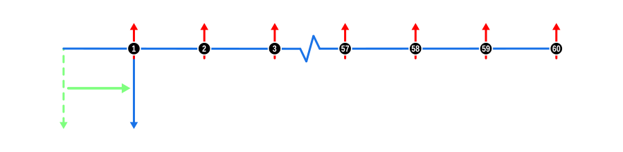
This example shows how to calculate a payment considering a short deferral of the amount due to an equipment supplier under a finance contract. This calculation is relevant for lenders with close ties to suppliers, allowing them to defer payments and pass on benefits like reduced payments or interest to borrowers. This technique is often used in competitive bidding where even slight interest rate reductions can be decisive. Note that borrowers and others using this calculator won’t know about this commercial relationship, so this example serves mainly for informational purposes.
This example illustrates how a lender can leverage a strong supplier relationship and make arrangements to defer settlement on equipment supplied to the borrower at the conclusion of a financing arrangement. In very many cases, the borrower is unaware of this arrangement, yet still enjoys the benefits of deferral in the form of a lower interest rate and reduced repayments.
Furthermore, this example demonstrates usage of the Deferred Settlements calculator feature to determine borrower repayments, using a lender’s desired return and taking into account the deferred settlement. In Examples 14 and 15, we show you how to calculate the Nominal Annual Rate (NAR) of interest implicit within the repayment profile from the Borrower and Lender perspective respectively. This feature is designed specifically for use by Finance Professionals, though the example should be informative for all users. The diagram below visualises the cash flow dynamics:
Example Calculation Inputs
Advance: The cost of the goods (advance) is shown as a blue downward arrow. In this example, the Advance arrow has been shifted from the start of the timeline, which is the Borrower’s perspective of the repayment profile, to the point in time the amount becomes due. This shift is illustrated by the light green arrow and reflects the financing arrangement from the Lender’s Perspective.
Payments: The unknown payments are represented by red upward arrows.
In the calculator input screen, at the foot of the Advances section, is a dropdown to select the perspective to use in solving the unknown payment value. As the lender is passing on the benefits of the deferral to the borrower, ensure the Lender’s Perspective option is selected so the calculation is performed with reference to the Settlement Date.
Benefits and Implications
For the Borrower:
Reduced Rates/Repayments: The deferral can result in lower interest rates or smaller payment amounts, making the financing more affordable or attractive.
Enhanced Affordability: Lower payments can make high-cost items more accessible or allow for better cash flow management.
Unaware Advantage: Borrowers benefit from the arrangement without needing to understand the underlying commercial relationships, potentially increasing their satisfaction with the financing terms.
For the Lender:
Maintains Yield: By deferring the settlement, the lender can maintain or even increase their yield without altering the interest rate visible to the borrower, as the cost savings from deferral are passed on.
Competitive Edge: This can be a strategic tool in competitive markets, allowing lenders to offer better terms without compromising their profitability.
Relationship Building: Strengthens ties with suppliers, which can lead to exclusive deals or better terms in future transactions.
For the Supplier:
Improved Stock Turnover: Deferring payment terms can help move inventory more quickly, especially for high-value or slow-moving items, reducing holding costs.
Sales Security: Securing sales under deferred terms is often preferable to keeping items in stock, potentially avoiding depreciation or obsolescence.
Market Positioning: Can position suppliers as flexible partners willing to negotiate terms to close deals, appealing to lenders and borrowers alike.
Cash Flow Management: While the payment is deferred, the sale is secured, allowing for better cash flow forecasting and management.
This deferred settlement scheme exemplifies how strategic partnerships can lead to mutual benefits, allowing for more cost-effective financing solutions while maintaining profitability and liquidity across the chain from supplier to lender to borrower.
Example 14
Determine a borrower’s NAR in a deferred settlement scheme
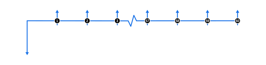
Expanding on Example 13, this example shows how to compute the borrower’s Nominal Annual Rate (NAR) of interest, similar to the IRR, in a deferred settlement scenario. Note that since payments factor in the deferral, the calculated NAR, based on the documented date, will likely be lower than the lender’s rate, as discussed in Example 15.
This example demonstrates usage of the Deferred Settlements calculator feature to illustrate how a lender can calculate the Nominal Annual Rate (NAR) of interest implicit in a repayment profile containing payments that already take into account the deferral of a supplier settlement. In Example 14, we illustrated how a Lender calculates this unknown payment value under a deferred settlement arrangement. In Example 15, we’ll show how a lender can confirm the Nominal Annual Rate (NAR) of interest implicit in a repayment profile aligns with the original yield used to calculate the unknown payment value.
The Deferred Settlement feature is designed specifically for use by Finance Professionals, though the example should be informative for all users. The diagram below visualises the cash flow dynamics:
Example Calculation Inputs
Advance: The cost of the goods (advance) is shown as a blue downward arrow. As this cash flow diagram shows the financial arrangement from the Borrower’s Perspective, the arrow is positioned at the beginning of the timeline.
Payments: The known payments are represented by blue upward arrows. In the calculator, enter the result obtained in Example 13 into the payment fields.
Interest Rate: As this is what we are solving, clear the calculator input field.
In the calculator input screen, at the foot of the Advances section, is a dropdown to select the perspective to use in solving the unknown interest rate. As we are determining the NAR from the Borrower’s Perspective, ensure that option is selected so the calculation is performed with reference to the Documented Date.
Note
We are describing the calculation of the implicit rate using the above approach as it is likely the calculator Display Settings are already set up and were used to calculate the unknown payment in the previous example. You can of course determine the implicit interest rate separately using the default calculator configuration as demonstrated in Example 16.
Benefits and Implications
Transparency: This calculation provides borrowers with a clear understanding of their effective interest rate, fostering transparency in financial dealings.
Comparison: Helps in comparing different financing options by understanding the true cost of borrowing under deferred settlement terms.
Example 15
Determine a lender’s NAR in a deferred settlement scheme
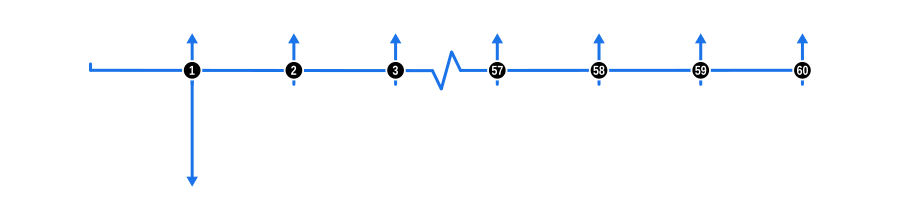
Building on Example 13 and linking to Example 14, this example shows how to compute the lender’s Nominal Annual Rate (NAR) of interest, similar to the IRR, in a deferred settlement scenario. The NAR calculation uses the settlement date, not the documented date, confirming that the lender’s rate or yield from Example 13 remains unaffected by the deferral.
This example illustrates the use of the Deferred Settlements calculator feature to verify that the Nominal Annual Rate (NAR) of interest implicit in a repayment profile, which accounts for the deferral of a supplier’s settlement, aligns with the original yield used to calculate the unknown payment value in Example 13. While Example 14 calculated the NAR from the borrower’s perspective, here we focus on the lender’s view to ensure financial consistency.
The Deferred Settlement feature is designed specifically for use by Finance Professionals, though the example should be informative for all users. The diagram below visualises the cash flow dynamics:
Example Calculation Inputs
Advance: The cost of the goods (advance) is shown as a blue downward arrow, located on the timeline when the supplier settlement occurs.
Payments: The known payments are represented by blue upward arrows. In the calculator, enter the result obtained in Example 13 into the payment fields.
Interest Rate: As this is what we are solving, clear the calculator input field.
In the calculator input screen, at the foot of the Advances section, is a dropdown to select the perspective to use in solving the unknown interest rate. As we are determining the NAR from the Lender’s Perspective, ensure that option is selected so the calculation is performed with reference to the Settlement Date.
Benefits and Implications
Verification of Yield: Ensures the lender’s expected return or yield is accurately reflected in the payment schedule, even after accounting for deferred settlements.
Financial Oversight: Provides a mechanism for lenders to double-check their financial models, ensuring all calculations align with their financial strategy.
Example 16
Determine the NAR implicit in a repayment schedule
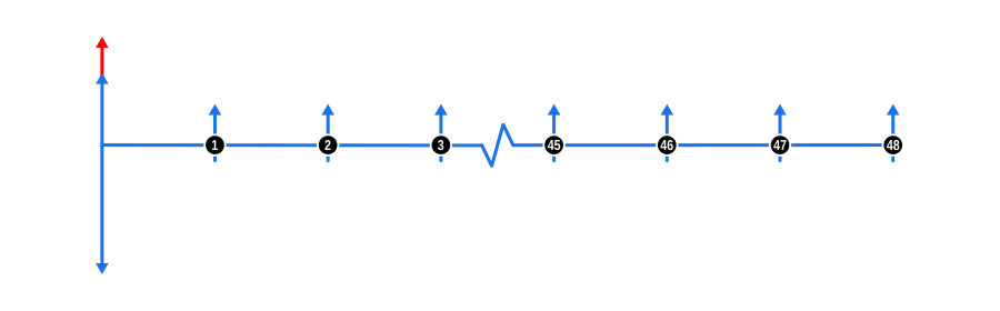
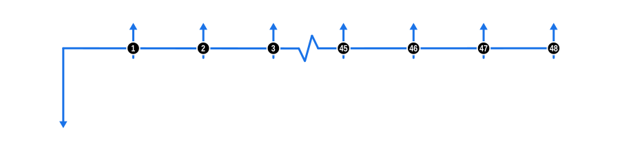
This example demonstrates how to calculate the Nominal Annual Rate (NAR) of interest, akin to the Internal Rate of Return (IRR), that’s inherent in a standard repayment schedule.
As an engaging exercise, cycle through various day count conventions to compute the implicit interest rate, and witness firsthand how different time interval measurements in each convention can dramatically impact the outcome.
Understanding the Nominal Annual Rate (NAR) is crucial for anyone dealing with finance, as it reveals the true cost of borrowing or the effective return on lending. This example serves as a foundational guide for calculating NAR in a repayment profile, equipping users with the knowledge to assess the economics of any loan or investment, from the simplest to the most complex structures.
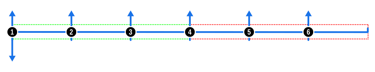
The diagram below visualises the cash flow dynamics of a standard repayment profile in Arrears:
Example Calculation Inputs
Advance: Depicted by a blue downward arrow at the start of the timeline, this represents the full cash price or loan value, known from the outset.
Payments: The blue upward arrows signify regular payments made in arrears, which means at the end of each payment period.
Interest Rate: Since we’re solving for this, ensure the calculator’s interest rate field is empty.
TIP
Once you’ve mastered these calculations, why not grab your local newspaper or visit finance websites to find loan advertisements? Use the details from these ads to input into the calculator and verify if the advertised interest rate holds up under scrutiny.
Also try sketching your own cash flow diagrams to capture the financial cash flows. You’ll find over time it is a great way to break down seemingly complex problems into a single well understood diagram.
Benefits and Implications
Transparency in Finance: Calculating NAR gives you a clear picture of the actual cost of borrowing or the yield on lending, promoting transparency in financial dealings.
Comparative Analysis: Use this skill to compare different financial products. Even small differences in NAR can lead to significant savings or costs over time.
Educational Value: This exercise is excellent for financial education, helping users understand how interest rates work across different conventions, which is vital when dealing with international finance where standards might differ.
Negotiation Tool: Armed with this knowledge, you’re better positioned to negotiate loan terms or investment opportunities, ensuring you’re not overpaying or undervaluing your financial engagements.
Spotting Discrepancies: By calculating NAR, you can quickly spot if an advertised rate doesn’t align with the repayment terms, which is crucial for consumer protection and informed decision-making.
This example not only sharpens your analytical skills but also empowers you to navigate the financial landscape with greater confidence and accuracy.
Example 17
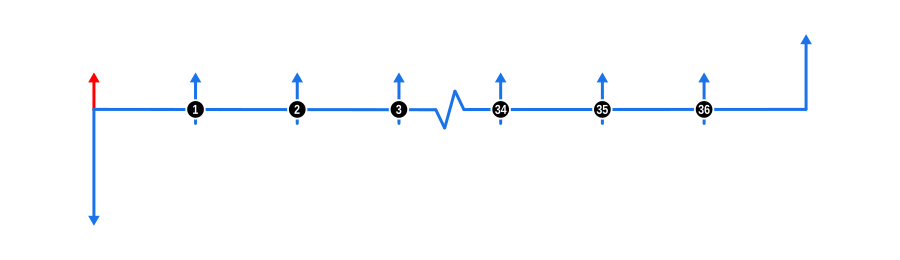
Determine the EAR implicit in a repayment schedule
This example demonstrates how to calculate the Equivalent Annual Rate (EAR) of interest inherent in a standard repayment schedule.
Note that all EAR day count conventions available in this calculator yield results comparable to legally defined Annual Percentage Rate (APR) conventions, making them excellent substitutes for APR calculations in jurisdictions without a defined APR standard.
This example illustrates the use of Effective Annual Rate (EAR) day count conventions and is included for the benefit of users outside the European Union who need a substitute method for calculating an Annual Percentage Rate (APR). The EAR conventions often mirror legally defined APR methods, providing a good proxy. Understanding the Effective Annual Rate (EAR) is crucial for anyone dealing with finance, as it reveals the true annualised cost of borrowing.
This example serves as a foundational guide for calculating EAR in a repayment profile, equipping users with the knowledge to assess the economics of any loan or investment, from the simplest to the most complex structures.
The diagram below visualises the cash flow dynamics of a standard repayment profile in Arrears:
Example Calculation Inputs
Advance: Depicted by a blue downward arrow at the start of the timeline, this represents the full cash price or loan value, known from the outset.
Payments: The blue upward arrows signify regular payments made in arrears, meaning at the end of each payment period.
Interest Rate: Since we’re solving for this, ensure the calculator’s interest rate field is empty.
TIP
This example does not incorporate Charge cash flows, which is something you may wish to do when determining the EAR implicit in a repayment profile. So, once you’ve mastered these calculations, why not add one or two charges and evaluate firsthand the impact a seemingly small charge has on the annual rate?
Benefits and Implications
Global Financial Literacy: Understanding EAR provides a universal language for discussing the cost of borrowing, especially useful in regions where APR isn’t standardised.
Accurate Comparison: Use EAR to accurately compare financial products from different countries or financial systems, ensuring you’re comparing apples to apples.
Consumer Advocacy: By calculating EAR, consumers can advocate for themselves, ensuring they’re not misled by nominal rates that don’t reflect the true cost of borrowing.
Financial Planning: Knowing the EAR helps in long-term financial planning, giving a clearer picture of how much borrowing will cost over a year, influencing decisions on loan terms or investment strategies.
Educational Tool: This example serves as an educational tool to understand how compounding affects the effective cost of loans, particularly when dealing with different compounding frequencies or additional fees.
This exercise not only enhances your ability to work with financial calculations but also deepens your understanding of how various elements of a loan or investment can impact your financial decisions.
Example 18
Determine the APR implicit in a repayment schedule, including charges
This example demonstrates how to calculate the Annual Percentage Rate (APR) for a consumer loan, in accordance with the European Union directive 2023/2225.
This example is invaluable for anyone dealing with consumer finance within the European Union, as it illustrates how to calculate the Annual Percentage Rate (APR) implicit in repayment profiles, including any charges. Understanding the APR is essential as it encapsulates the total cost of borrowing, providing a standardised metric for comparing different loans.
The diagram below visualises the cash flow dynamics of a standard repayment profile in Arrears, including a single charge:
Example Calculation Inputs
Advance: Depicted by a blue downward arrow at the start of the timeline, this represents the full cash price or loan value, known from the outset.
Payments: The blue upward arrows signify regular payments made in arrears, meaning at the end of each payment period. The large blue upward arrow coinciding with the final payment represents a balloon payment, often used to align with the residual value of an asset or to defer a significant portion of the repayment.
Charges: There is one charge due at the outset of the contract, represented by a green up arrow, which could include fees like an origination fee or setup costs.
Interest Rate: Since we’re solving for this, ensure the calculator’s interest rate field is empty.
TIP
When you’re comfortable determining the APR implicit in a repayment profile, why not get a little more creative? Did you know Curo Calculator can be used to determine an unknown value in a repayment profile that includes charges, ensuring an exact APR yield is obtained? It can, so try it out!
Benefits and Implications
Consumer Protection: By calculating the APR, consumers can make informed decisions, ensuring they understand the full cost of loans, including all associated charges.
Regulatory Compliance: This example adheres to EU standards, helping financial institutions comply with consumer credit directives, ensuring transparency in lending practices.
Loan Comparison: APR is a universal measure for comparing different loan offers, especially when they include various fees or charges, making it easier to choose the most cost-effective option.
Financial Literacy: Educates users on how charges affect the overall cost of borrowing, promoting better financial decision-making.
Negotiation: Knowing how to calculate APR gives borrowers leverage in negotiations, particularly when discussing how fees and charges should be structured or reduced.
Business Decisions: For businesses offering credit, understanding how to calculate APR ensures they can price their loan products competitively while still covering costs and maintaining profitability.
This example not only teaches you to compute APR but also highlights its importance in the broader context of consumer finance within the EU, empowering both lenders and borrowers to navigate the financial landscape more effectively.
Core Concepts
Dive into the heart of financial calculations with this section of the guide. Here, we unpack several pivotal financial concepts, illustrating how they’re woven into the fabric of Curo Calculator. Explore these essential topics:
Day Count Conventions: Grasp the significance of how days are counted in financial calculations. Learn about key conventions like 30/360 for standard loan calculations, Actual/Actual for precision over long terms, and Actual/365 for short-term finance. Understand when to apply APR conventions for consumer credit, and how EAR conventions annualise rates for broader applicability.
Interest Rates: Delve into the nuances of interest calculations with Nominal Annual Rate (NAR) as the basic yearly rate, Effective Annual Rate (EAR) which accounts for compounding, and Annual Percentage Rate (APR) which includes additional borrowing costs like fees, providing a legal standard for comparing loan costs. Understand how the day count convention you select influences which rate type is used in your calculations.
Modes: Understand how the timing of payments within a period affects your calculations. Learn to differentiate between In Advance (payments at the start of periods) and In Arrears (payments at the end), and see how consistent or mismatched modes across multiple payment or charge rows influence cash flow patterns.
Schedules: Explore the Amortisation Schedule for a clear breakdown of loan payments, showing how each instalment reduces principal and pays interest, ideal for financial accounting. Alternatively, the EAR/APR Proof schedule validates the calculated interest rate by ensuring discounted cash flows balance to zero, crucial for rate accuracy verification. Both schedules can be downloaded in XLSX format, with options to view day count factors for deeper analysis.
Embark on this journey through Curo Calculator’s core concepts to enhance your financial acumen and make the most of your calculations.
Subsections of Core Concepts
Day Count Conventions
Quick Version
A Day Count Convention is essentially a method of counting days for financial calculations. It might sound complex, but it’s really just about counting days in different ways.
Choosing the right convention for your calculation can be confusing due to the various options available. However, most loan repayment calculations use a limited subset of conventions available in Curo Calculator, with others reserved for more specialised scenarios. If you’re looking for guidance on which to use, here are our recommendations:
Solving unknown values and implicit interest rates:
For calculations with repayments in months or multiples of months, use 30/360. This convention is often considered the de facto standard for many financial calculations and has been in widespread use for decades.
For calculations with repayments in weeks or multiples of weeks, opt for Actual/365 or Actual/Actual. Avoid conventions based on a 30-day month as these might yield unexpected results due to how they handle periods spanning month ends.
Solving unknown APRs and unknown values using an APR:
For users in the European Union (EU), use the built-in EU 2023/2225 APR convention.
For users in the United States (US), use the built-in US Appendix J APR convention.
For users in the United Kingdom (UK), select the UK Mortgage APR for credit agreements secured on land or UK Non-Mortgage APR for those not secured on land.
For users located elsewhere, choose conventions with the EAR (Effective Annual Rate) suffix, e.g., 30/360 EAR. These conventions often mirror legally defined APR methods, providing a good proxy. If your jurisdiction has a mandated APR convention, please let us know, and we’ll consider adding support in a future release.
Continue reading for a deeper understanding of Day Count Conventions in general.
Deep Dive Version
All conventions supported by Curo Calculator are listed below, each with details to help you select the most appropriate one for your needs.
Each standard convention has a counterpart EAR (Effective Annual Rate) convention, which isn’t described separately as they use the same method of counting days. They differ only in where they start the day count from; in standard conventions, the count is based on the duration between the current and previous cash flow. In the EAR version, the count is the duration between the current and the initial advance or drawdown. This method effectively annualises the interest rate.
Info
If you work with spreadsheets, you might be familiar with the IRR (Internal Rate of Return) and XIRR (eXtended Internal Rate of Return) functions. The good news is Curo Calculator produces identical results when you solve for the unknown rate using 30/360 for IRR calculations, and Actual/365 EAR or Actual/Actual EAR for XIRR calculations!
One final point: No matter which convention you use, it’s very easy to inspect the day counts applied to each cash flow in a repayment schedule. This way, you can sense-check if your chosen convention is working as expected. For further information, see Core Concepts > Schedules.
Here are the supported conventions:
EU 2023/2225 APR
Description:
This convention expresses time intervals in years, months, or weeks, considering the frequency of drawdowns and payments.
Mathematical Logic:
When intervals can’t be expressed in whole periods, the remaining days are calculated backwards from the cash flow date to the initial drawdown, divided by 365 (or 366 in a leap year).
Use Cases:
Mandatory for computing the Annual Percentage Rate of Charge (APRC) for Consumer Credit in the EU.
Historical Context:
Implemented with the EU’s Consumer Credit Directive 2023/2225.
Example:
Weekly: From January 1 to February 4 would be counted as 5 weeks (divided by 52 weeks in a year).
Monthly: From January 1 to March 1 would be counted as 2 months (divided by 12 months in a year).
US Appendix J APR
Description:
This convention calculates the Annual Percentage Rate (APR) for closed-end credit transactions using the actuarial method, where time intervals are determined by the user-selected repayment frequency (e.g., weeks, months, or multiples thereof), with any remaining days counted as a fraction of a year.
Mathematical Logic:
Intervals are measured based on the repayment frequency chosen by the user:
For weekly payments, intervals are counted in weeks (divided by 52 for the year fraction).
For monthly payments, intervals are counted in months (divided by 12 for the year fraction).
For other frequencies (e.g., semi-monthly or multiples of weeks/months up to one year), the unit-period is the most frequent common period in the transaction.
If the interval includes a partial period (odd days), the remaining days are counted as the actual number of 24-hour intervals between dates, divided by 365, regardless of leap years.
The day count starts from the transaction’s consummation date (or when the finance charge begins, if later) to each cash flow, using the actuarial method where the unpaid balance is increased by the finance charge and decreased by payments at the end of each unit-period.
Use Cases:
Mandatory for calculating the APR for consumer credit agreements in the United States, including loans, credit cards, and other closed-end credit transactions, as required by Regulation Z of the Truth in Lending Act (TILA).
Historical Context:
Established under Appendix J of Regulation Z, part of the U.S. Truth in Lending Act (TILA), to standardize APR calculations for consumer transparency, effective since the TILA’s enactment in 1968 and refined through subsequent amendments.
Example:
Weekly: For a transaction from January 1 to February 5 (35 days, or 5 weeks), the interval is counted as 5/52 years, with no odd days if payments align weekly.
Monthly: For a transaction from January 1 to March 10 (68 days), if monthly payments are selected, the interval is counted as 2/12 years (for two months) plus 10/365 years (for the remaining 10 days).
UK Mortgages APR (UK CONC App 1.1)
Description:
This convention is used for calculating the Annual Percentage Rate of Charge (APRC) specifically for consumer credit agreements secured on land in the United Kingdom.
Mathematical Logic:
Periods are measured in whole calendar months or weeks when possible. For periods that don’t align with whole months or weeks, time is converted into years and days.
Whole months or weeks are converted to years; any remaining days are expressed as a fraction of a year based on the year’s actual number of days (365 or 366 for leap years).
Use Cases:
Essential for mortgages and other credit agreements where the security is land in the UK.
Historical Context:
Derived from the UK’s Financial Conduct Authority (FCA) Consumer Credit sourcebook (CONC), specifically Appendix 1.1.
Example:
If a period spans from January 1 to April 1, it would be counted as 3 whole months (divided by 12 for the year fraction), or if from January 1 to January 29, it might be considered as 29 days (divided by 365 or 366 for a year fraction).
UK Non-Mortgages APR (UK CONC App 1.2)
Description:
This convention applies to calculating the Annual Percentage Rate of Charge (APRC) for consumer credit agreements not secured on land in the United Kingdom.
Mathematical Logic:
Time intervals between dates are calculated directly in years or fractions thereof.
A year can be viewed as having 365 days (or 366 in leap years), 52 weeks, or 12 equal months.
For irregular periods, the time is converted into a fraction of a year based on the number of days in the year (365 or 366 for leap years).
Use Cases:
Applicable for various forms of consumer credit like loans, credit cards, etc., where no land is involved as security.
Historical Context:
Also part of the UK’s FCA CONC sourcebook, with specifics in Appendix 1.2.
Example:
From January 1 to January 31 would be 31 days, considered as a fraction of 365 (or 366 in a leap year) for the year. If from January 1 to March 1, it would be counted as 2 months (divided by 12 for the year fraction), or alternatively, as 59 days.
30/360 Convention
Description:
Assumes each month has 30 days and each year has 360 days for simplified calculations.
Mathematical Logic:
Days are calculated as if every month ends on the 30th, regardless of actual days.
Use Cases:
Preferred for bonds, fixed income, and standard loan calculations for its simplicity.
Historical Context:
Developed for manual calculations before widespread computer use.
Example:
Interest from January 1 to March 1 counts as 60 days (2 months x 30 days).
Actual/Actual (ACT/ACT) Convention
Description:
Uses the actual number of days between dates and accounts for leap years.
Mathematical Logic:
Counts every actual day, dividing by the year’s actual number of days (365 or 366).
Use Cases:
Essential for precise interest calculations in government bonds and long-term securities.
Historical Context:
Chosen for markets requiring accuracy over long periods.
Example:
From January 1, 2024, to January 1, 2025, would be 366 days if it’s a leap year.
Actual/365 (ACT/365) Convention
Description:
Counts actual days but uses a fixed 365-day year, ignoring leap years.
Mathematical Logic:
Interest is calculated over actual days but with a constant year length.
Use Cases:
Used in money markets, commercial loans, where leap years are less critical.
Historical Context:
Designed for consistent annual rate calculations in short-term finance.
Example:
From January 1 to June 1 counts over 365 days, regardless of leap years.
Actual/360 (ACT/360) Convention
Description:
Employs actual days but assumes each year has 360 days for calculations.
Mathematical Logic:
Results in higher annualised rates due to the smaller denominator.
Use Cases:
Common in U.S. banking for short-term debt where a higher annual rate is acceptable or required.
Historical Context:
Adapted from European practices for U.S. markets.
Example:
From January 1 to January 31 counts as 31 days over 360, leading to a higher annual percentage rate compared to 365 or 366 days.
Interest Rates
Quick Version
Curo Calculator is designed to solve unknown values using one of three rates of interest: a Nominal Annual Rate (NAR), an Effective Annual Rate (EAR), and an Annual Percentage Rate (APR). It also solves for an unknown interest rate when all other inputs are provided.
The type of interest used in a calculation is determined by your choice of day count convention. See Core-Concepts > Day Count Conventions for details on supported conventions. When selecting a convention on the calculator input screen, you’ll notice the label of the interest rate input field updates to reflect the type of interest that will be used.
Nominal Annual Rate (NAR) - The basic interest rate over a year without considering compounding or inflation.
Effective Annual Rate (EAR) - Takes into account the effect of compounding within the year, giving a more accurate annual rate.
Annual Percentage Rate (APR) - Similar to EAR in calculating days with reference to the initial drawdown but mandated by law to reflect the true cost of borrowing, including fees and other charges, but not considering compounding frequency within the year.
Deep Dive Version
Nominal Annual Rate (NAR)
Definition: The NAR is the stated interest rate for a year, before adjustments for compounding or inflation. It’s the simplest form of expressing interest.
Example: If a loan has a NAR of 5%, this means you would pay 5% of the principal in interest over one year, if no compounding is applied.
$$ Interest = Principal \times \frac{NAR}{100} $$
Effective Annual Rate (EAR)
Definition: The EAR accounts for the effects of compounding within the year. It’s the actual rate you would pay or earn annually, considering how often interest is compounded.
Example: For a nominal rate of 5% compounded quarterly:
Definition: The APR is a standardised measure of the cost of borrowing, mandated by law to reflect not just the interest rate but also other charges like fees, providing a more comprehensive view of borrowing costs. However, unlike NAR, it does not account for the frequency of compounding within the year.
Example: Consider a one-year loan of €1,000 where:
The Nominal Annual Rate (NAR) is 5%.
The loan has an origination fee of 1% (€10 added to the cost).
Interest compounds monthly, but for simplicity, we’ll calculate APR assuming annual compounding for comparison with regulatory standards.
Calculating APR:
Total Interest: Based on NAR, the interest would be €1,000 * 5% = €50.
Total Fees: The origination fee adds €10.
Total Cost of Borrowing: €50 (interest) + €10 (fee) = €60.
For APR:
Simplified APR Calculation (assuming annual compounding for regulatory purposes):
This means, although the NAR is 5%, when you include the fee, the APR effectively becomes 6%, providing a clearer picture of the loan’s cost without considering the compounding effect within the year.
Modes
A mode determines when an amount is due within the period defined by a chosen frequency. With a mode set to In Advance, the amount becomes due at the start of the first period, and in any subsequent periods within a cash flow series. When set to In Arrears, the amount is due at the end of the first and subsequent periods.
Note
When set to In Advance, a single payment or charge is automatically assigned a One-off frequency, occurring as a single event without recurring periods. This aligns the cash flow with the contract start date or the end date of a prior series for improved readability. Explore this feature in examples 02, 05, and 11.
The Mode selection is only displayed when date input is disabled, a topic covered in Settings > Display > Date Input. When dates are in use, you have full control over when the first amount in a series falls due.
Modes with Multiple Rows
When performing calculations with more than one Payment or Charge, the mode you select in each row applies only to that row. To avoid unexpected results from mismatched modes, as described below, you should aim for consistency by using the same mode across all Payment or Charge rows.
The first diagram illustrates the consistent application of the In Advance mode across two payment series, resulting in equal spacing of cash flows. This spacing would be similar if both were set to In Arrears.
The next diagram shows the effect when the first payment series is set to In Advance and the second to In Arrears. The mismatch results in a gap, the width of which is equal to the frequency of each series.
Conversely, the following diagram depicts what happens when the first payment series is In Arrears and the second is In Advance. Here, the final payment in the first series coincides with the first payment of the second.
Keep these points in mind when selecting modes across multiple rows to ensure your calculations align with your expectations.
Schedules
Curo Calculator offers two distinct types of schedules: the Amortisation Schedule and the EAR/APR Proof. The choice of day count convention you make on the input dictates which schedule will accompany your calculation results, accessible on the second tab of the results screen. Here’s the breakdown:
Amortisation Schedule: Generated for all standard day count conventions (e.g., 30/360, Actual/Actual), this schedule details each payment on a loan, showing how each instalment is split between interest and principal reduction. This is particularly beneficial for business borrowers who need to update their financial accounts with precise payment allocations.
EAR/APR Proof: Produced when using conventions with an EAR or APR suffix (e.g., US Appendix J APR, EU 2023/2225 APR), this schedule demonstrates the calculation methodology behind the rate and verifies its accuracy by ensuring that all discounted advances, payments, and charges net out to zero. It’s invaluable for both lenders and borrowers who need to validate or dispute the interest rate applied to a loan.
From a Curo Calculator perspective, these schedules serve to:
Present results in an easily digestible format.
Allow you to quickly sense-check if your calculation inputs yield the expected repayment profile, particularly in complex scenarios with multiple variables.
Enable validation of an interest rate result when necessary.
All schedule data can be downloaded in XLSX (spreadsheet) format for your records or further analysis. Simply click the download button at the top of each schedule.
When a schedule contains same-dated payments, a Bundle Payments button appears at the top. Toggle this button to bundle or unbundle same-dated payments for a cleaner, more organized display. Explore this feature in examples 07 and 09.
The following section delves into how to validate any interest rate result produced by Curo Calculator using the data provided in these schedules. This part gets quite technical and might primarily interest those seeking a deep dive.
Interest Rate Validation
EAR/APR Proof
The EAR/APR Proof schedule uses one of two discount approaches to validate the interest rate, depending on the selected APR convention:
Standard APR Conventions (e.g., EU 2023/2225 APR): These use a standard discount formula and display a Discount Inputs column with the factor ( $t$ ) for each row.
US Appendix J APR: This uses a U.S.-specific discount formula, reflecting the actuarial method, and displays a Discount Inputs column with parameters ( $f$ ), ( $t$ ) and ( $p$ ) for each row.
Below, we provide a simplified example for each approach to illustrate the validation process.
Standard APR Conventions
For standard APR conventions, the proof schedule includes a Discount Inputs column showing ( $t$ ), the time factor for discounting. Below is an example schedule:
The interest rate to validate is found under the result summary tab:
To prove the interest rate (5.11%) is accurate, discount each value in the Amount column using the Discount Inputs ( $t$ ) and the annual interest rate (as a decimal), then sum the results. The discount formula and example calculations are provided below:
Standard APR discount formula
$$ d = a \times (1 + i)^{-t} $$
where:
( $d$ ) = Amount Discounted
( $a$ ) = Amount (to be discounted) from the schedule
The Balancing Total column maintains a running total that should reduce to zero, though minor variations (±0.01) may occur due to rounding. Here, the total is -0.00, confirming the interest rate of 0.05106868 (5.11%) is correct for the EU 2023/2225 APR convention.
US Appendix J APR
For the US Appendix J APR convention, the proof schedule includes a Discount Inputs column showing ( $f$ ) (odd-days factor), ( $t$ ) (unit-period time factor) and ( $p$ ) (unit-periods in a year). Below is an example schedule for a loan with three monthly repayments:
The interest rate to validate is found under the result summary tab:
To prove the interest rate (4.99% annual) is accurate, discount each value in the Amount column using the Discount Inputs ( $f$ ), ( $t$ ), ( $p$ ) and the annual interest rate ( $i$ ) (expressed as a decimal), then sum the results.
The discount formula and example calculations are provided below:
US Appendix J APR discount formula
$$ d = \frac{a}{(1 + f\frac{i}{p})(1 + \frac{i}{p})^t} $$
where:
( $d$ ) = Amount Discounted
( $a$ ) = Amount (to be discounted) from the schedule
The Balancing Total column maintains a running total that should reduce to zero, though minor variations (±0.01) may occur due to rounding. Here, the total is -0.00, confirming the annual interest rate of 0.04991094 (4.99%) is correct for the US Appendix J APR convention.
Amortisation Schedule
To validate the interest rate, we offer a simplified example of an amortisation schedule in the image below:
Notice the additional column after the Date column, which shows the Discount Inputs applied to each row. This column is hidden by default because day count factors can be confusing. To view it, tap or click 3 times on the Date column title. Repeat to hide it again.
The interest rate you need to validate can be found under the result summary tab:
To confirm that the interest rate of 4.99% (as shown above) is accurate, you need to calculate the periodic interest for each row. Add this interest to the capital balance brought forward and the amount to determine the capital balance carried forward. Repeat this for each row until you reach the end.
Here’s the formula for periodic interest, followed by the step-by-step workings:
In amortisation calculations, the final Capital Balance should ideally be zero, with minor deviations permitted due to rounding errors, thus proving the interest rate of 0.04991095 (4.99%) correct for the chosen 30/360 day count convention.
Tip
Even if you’re not interested in validating the interest rate, uncovering the Discount Inputs column can be helpful to see how the day counts are used in the calculation for your selected convention. Remember, the day count is based on the duration between the current and previous cash flow.
Blog Posts
Subsections of Blog Posts
Multiple Interest Rate Calculations
As outlined in the introduction to this help guide, Curo Calculator does not support calculating unknown values in scenarios where interest rates change over time, like in fixed-to-variable rate mortgages, in a single step. However, you can perform these calculations by breaking them down into several steps. We’ll demonstrate this process using the default settings in Curo Calculator, concluding with how to calculate the Nominal Annual Rate (NAR) and Annual Percentage Rate (APR) implicit in the entire repayment schedule.
Fixed-to-variable rate lending is predominantly used within the mortgage industry. We’ll use a real-life example from an Irish mortgage lender to illustrate this concept. Typically, all necessary inputs are provided, but be ready to search for them if they aren’t. Here’s what you’ll need:
Loan amount
Fixed rate of interest
Fixed repayment term
Total repayment term
Variable rate of interest
Fixed-to-Variable Interest Rate Mortgage Example
Fixed Rate Representative Example: €300,000 loan repayable over 30 years term, first five years fixed. Fixed rate of interest 4.50% per annum and 4.11% APRC*. 60 monthly repayments of €1,520.06 per month. On the expiry of a fixed rate period, your mortgage account will revert to a variable rate in accordance with the terms of your loan documentation for the remaining 300 months.
Variable Rate Representative Example: €300,000 loan repayable over 30 years. Rate of interest 3.85% per annum variable. 3.92% APRC*. 360 monthly repayments of €1,406.42 per month. Total amount payable is €505,718.08.
In the lender example above, the fixed repayment value of €1,520.06 per month is provided. This is not always the case, so we’ll start off showing how to calculate it.
Step 1: Determine/Confirm the fixed-rate repayment value
To calculate the unknown fixed repayment, we treat the entire 30-year term as the fixed repayment period and use the fixed rate of interest in the calculation. The required inputs are as follows:
Advances Amount: Enter the loan of €300,000.00
Payments: Ensure the payment row has the following inputs/selections:
Number of: 360
Frequency: Monthly
Amount: Leave blank as we are calculating this
Mode: In Arrear
Day Count Convention: Select the 30/360 (this convention assumes each month has 30 days and each year has 360 days for calculation purposes)
Nominal Annual Rate: Enter the fixed rate of 4.50%
Once done, the inputs should match the image below.
After pressing the Calculate button, make a note of the payment result as we use this as input in Step 2.
Step 2: Determine the fixed-rate period end balance
To calculate the value of the variable rate repayments, we first need to determine the capital balance outstanding at the end of the five-year fixed term. To do so, amend the calculator input as follows:
Payments: In the payment row from Step 1, leave everything as is except for:
Number of: Change from 360 to 60
Amount: Enter the payment value result (€1,520.06) from Step 1
Now select the ‘Add row’ link below the previous row, which we’ll use to calculate the balance after 5 years:
Number of: Enter 1
Frequency: leave as ‘Monthly’
Amount: leave blank as this is what we are calculating
Mode: Here, we use ‘In Advance’ because we’re calculating the balance after the last fixed payment has been made
When you are done, your calculator input will be the same as shown below.
After pressing the Calculate button, make a note of the result as we use this as input in Step 3.
Step 3: Determine the variable-rate repayment value
Now that we know the balance at the end of the fixed term, we can calculate the variable-rate repayments for the remaining 25 years. First, remove the second payment series row we added in Step 2, as it was only needed for calculating the balance after the fixed term. Then, use the following inputs:
Advances Amount: Enter the balance from Step 2 as the new loan amount (€273,473.48).
Payments: With the second row removed, amend the remaining payment row as follows:
Number of: 300 (since 360 total months minus 60 fixed months)
Frequency: Monthly
Amount: Leave blank to calculate
Mode: In Arrear
Day Count Convention: Select 30/360
Nominal Annual Rate: Enter the variable rate of 3.85%
After calculating, make a note of this new repayment amount for the last step.
Step 4: Determine the NAR and APR implicit in the schedule
To calculate the NAR and APR it’s probably wise to clear all calculation inputs and start with a clean slate. Whatever route you take the required inputs are as follows:
Advances Amount: Enter the loan of €300,000.00
Payments:
Row 1: Ensure the payment row has the following inputs/selections:
Number of: 60
Frequency: Monthly
Amount: €1,520.06
Mode: In Arrear
Row 2: Add another row and ensure it has the following inputs/selections:
Number of: 300
Frequency: Monthly
Amount: €1,420.94
Mode: In Arrear
When you are done, your calculator input will be the same as shown below.
To calculate the NAR:
Day Count Convention: Select the 30/360
Nominal Annual Rate: Leave blank as this is what we are to calculate
To calculate the APR:
Day Count Convention:
Select EU 2023/2225 APR for European Union mortgages
Select UK Mortgage APR for United Kingdom mortgages
Select 30/360 EAR as a proxy in other parts of the world
Annual Percentage Rate: Leave blank as this is what we are to calculate
By following these steps, you can now use Curo Calculator to effectively manage and analyse fixed-to-variable rate mortgage scenarios. Understanding how to break down these calculations into manageable steps not only aids in financial planning but also gives you a clearer picture of the long-term implications of varying interest rates on your repayments. Remember, while Curo Calculator simplifies these processes, real-world applications might require additional considerations like fees, insurance, or changes in policy that could affect your mortgage. Keep this guide handy as a reference, and always consult with a financial advisor for personalised advice tailored to your specific circumstances.
Need More Help?
Try these next steps:
Contact Us Directly
For technical issues, feature requests, or to report bugs, email us at curocalculator@gmail.com. We aim to respond quickly.
Check Out The Code
Interested in the calculations behind the app? The financial calculation library that powers Curo Calculator was open-sourced under an MIT License and is available on GitHub.